Depth articles - History of Target Detection (D) from the elaborate to the Fast R-CNN target detection Faster R-CNN

Returns the directory object detection history

Previous: depth articles - Target Detection History (c) elaborate SPP-Net Target Detection

Next: depth articles - Target Detection History (five) elaborate SSD target detection

Paper Address: "Fast R-CNN" , "Faster R-CNN"

Code Address: Faster-rcnn

In this section, from the elaborate to the Fast R-CNN Faster R-CNN object detection, object detection in the next section elaborate SSD

Four. Fast R-CNN target detection (2015)

To solve the problem of double counting R-CNN and SPP-Net brings about 2k a bounding boxes, so R-CNN authors developed a Fast R-CNN.

1. Fast R-CNN main idea

(1) using a simplified layer SPP

Use ROI pooling layer, and the operation is similar to SPP

(2) The training and testing is no longer in several steps

No additional hard disk to store features of the intermediate layer, a gradient layer can be spread by pooling the linear ROI. In addition, classification and regression together with Multi-task way

(3). SVD

Using full-matrix parameters of the SVD connection layer, two small-scale compression many fully connected layer.

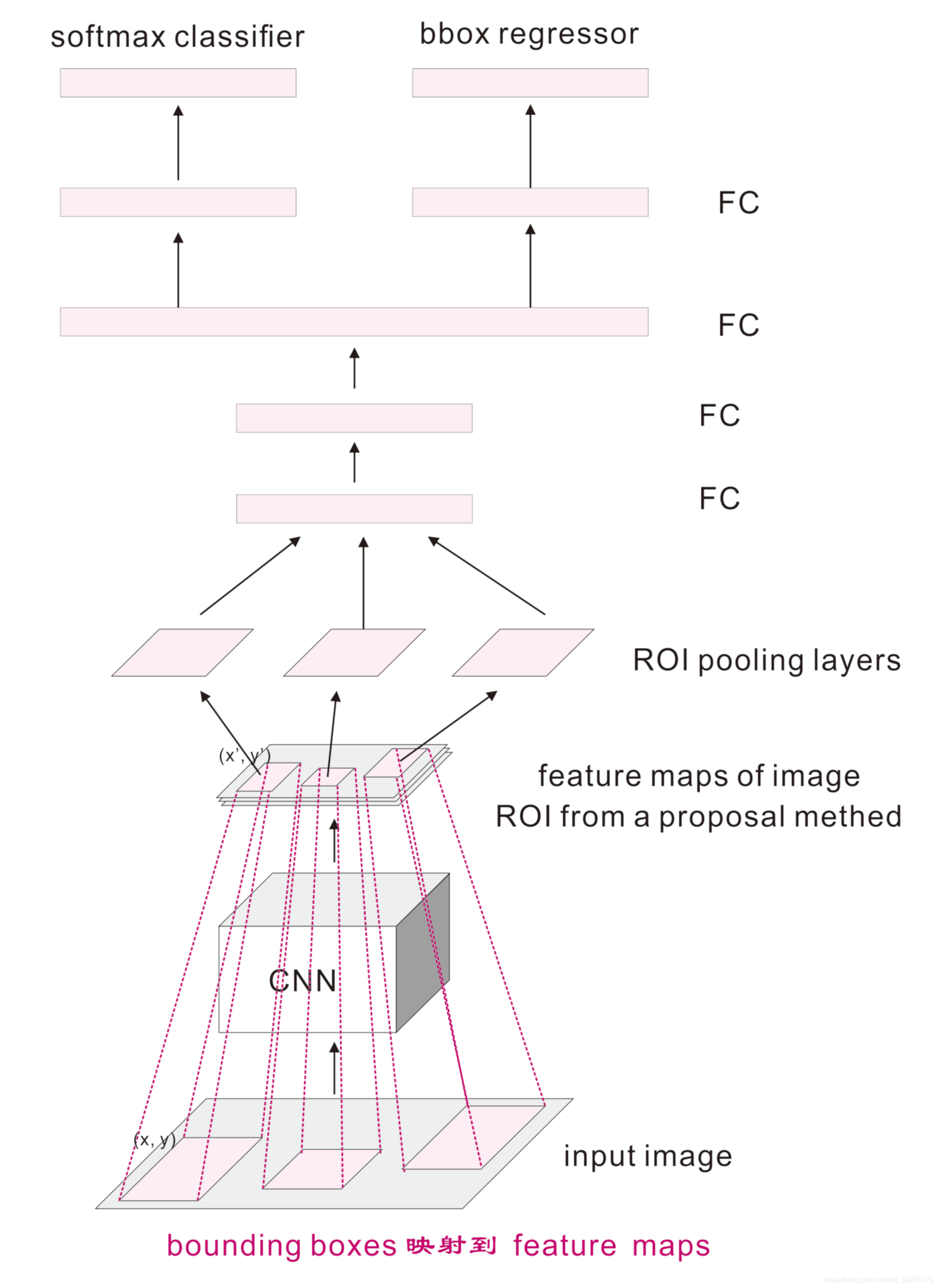
2. Fast R-CNN main steps

(1). Region proposal to nominate area

Region proposal bounding boxes extracted from an original image by a method such as selective search

(2). Feature extraction

The whole image is input to the CNN network, obtain the relevant feature maps

(3) mapping

The bounding boxes to the last one mapping feature maps on

(4) The area normalized

Perform ROI pooling operation region proposal bounding boxes for each of the feature maps (this process is similar to a simplified version of the operation layer SPP) to give a fixed size of feature maps.

ROI pooling of specific operations, can refer back to what I wrote: depth articles - CNN convolutional neural network (C) ROI pooling and ROI Align interpolation on

(5) Classification and Regression

Then through two fully connected layers, multi-target detection softmax classification respectively (here made significant changes had previously been done by SVM classification), fine-tune the location and size of the border with the regression model.

SPP-Net is a good way, R-CNN advanced to Fast R-CNN is adopted on the basis of R-CNN on the SPP-Net method, R-CNN has been improved so that performance can be further improved. Fast R-CNN in fact replace the SPP layer with ROI pooling, replace the SPP-Net SVM with multi-task loss.

3. Fast flowchart of R-CNN

Multitasking 4. Fast R-CNN loss of function

(1). Fast R-CNN has two output loss result

. (2) The output is a discrete probability distribution (for each ROI), for Category k + 1 (k is an object classification of the ROI, a background) are: $\large p = (p_{0},\; ......,\; p_{k})$

(3) The other output is compensated return bounding boxes (bounding boxes regression effsets). For the k th target in the target class for each class k are: $\large t^{k} = (t_{x}^{k},\; t_{y}^{k},\; t_{w}^{k},\; t_{h}^{k})$

(4) The use of more than one task at a loss on the ROI of each tag L to joint training for classification and regression bounding boxes.

$\LARGE L(p, \mu, t^{\mu}, v) = \left\{\begin{matrix} L_{cls}(p, \mu) + \lambda L_{loc}(t^{\mu}, v) & (\mu \; is \; foreground) \\ L_{cls}(p, \mu) & (\mu \; is \; background) \end{matrix}\right.$

$\LARGE L_{cls} (p, \mu) = -log_{2} p_{\mu}$

$\LARGE L_{loc}(t^{\mu}, v) = \sum_{i \in (x, y, w, h)} smooth_{L_{1}} (t_{i}^{\mu} - v_{i})$

$\LARGE smooth_{L_{1}} (x) = \left\{\begin{matrix} 0.5 x^{2} & |x| < 1 \\ |x| - 0.5 & |x| \geq 1 \end{matrix}\right.$

$\large \mu$ : Training ROI for each corresponding to a ground truth, it is divided into foreground and background

$\large v$ : A ground for the real truth of coordinates, $\large v = (v_{x},\; v_{y},\; v_{w},\; v_{h})$

$\large t^{\mu}$ : For the first $\large \mu$ return compensation bounding boxes of the target class, $\large t^{\mu} = (t_{x}^{\mu},\; t_{y}^{\mu},\; t_{w}^{\mu},\; t_{h}^{\mu})$

$\large p$ : Do softmax for each ROI k + 1 classification probability calculated, $\large p = (p_{0}, p_{1}, ......, p_{k})$ . This k + 1, where k is the k th target classification, a classification for the background.

$\large L_{cls}(p, \mu)$ : For the first $\large \mu$ category of the real number of losses (cross-entropy)

$\large L_{loc}(t^{\mu}, v)$ : For each $\large \mu$ of the tuple prediction $\large t^{\mu} = (t_{x}^{\mu},\; t_{y}^{\mu},\; t_{w}^{\mu},\; t_{h}^{\mu})$ and the real coordinate tuple corresponding ground truth $\large v = (v_{x},\; v_{y},\; v_{w},\; v_{h})$ lost.

$\large L_{1}$ : A strong $\large L_{1}$ loss, less sensitive to outliers (used in the R-CNN and SPP-Net $\large L_{2}$ Loss)

$\large \lambda$ : Ultra parameter to balance the two loss function. Of ground truth normalized return target $\large v_{i}$ mean and unit variance are zero, and are used in these experiments $\large \lambda = 1$ .

5. Fast R-CNN VS R-CNN & SPP-Net

Since Fast R-CNN is the entire input image is an image CNN operation, ROI pooling and used so that the efficiency, faster than R-CNN and SPP-Net, R-CNN crop and does not result in warp or error. Furthermore, Fast R-CNN used softmax alternative SVM, so that better efficiency classification model training and testing, and the results would be significantly improved. For the limited data, the use of SVM will have better, however, when the user has to do massive data model, SVM situation is very embarrassing. Because it is calculated is the goal of a separate calculated, rather than softmax, it is calculated together; it also results in a relatively large number of classification categories time, SVM model will be relatively large.

Five. Faster R-CNN target detection (2015)

1. Fast R-CNN using selective search to nominate area, speed is still not fast enough. Faster R-CNN bounding boxes calculated directly using RPN (Region Proposal Networks, RPN) network. RPN an image to any size of the input and output number of the rectangular area nominated each corresponding to a target classification and position information.

2. RPN nominated area network

RPN output is a set of boxes / proposal, classification and regression is will these boxes / proposal inspection, final inspection occurs where the target is. More precisely, RPN network is forecasting an anchor foreground or background, and the anchor has been refined.

(1). Specifically RPN network

①. RPN added after the last convolution network layer, sliding window on feature maps.

②. To build a neural network regression object classification + box location

Position ③. Slide window, there is provided a general position information of the object

④. Return box provides a more precise location of the box

⑤. By the trained bounding boxes region.

(2). Foreground and background classifier

Training a classifier first step is to establish a training data set, the training data set is RPN process and those ground truth boxes to mark all of the anchors. The basic idea is: desirable to have a higher labeled as foreground overlapping anchors, anchors having a lower overlapping labeled background. Obviously, this requires some adjustments and compromises to separate foreground and background. In reality, these details can be queried, so there will be anchors mark.

(3). Feature on anchors at

For example, 600 x 800 image after application of CNN, flashes once every 16 steps, to give 1989 (39 x 51) feature maps. In this 1989 feature maps, each location has nine anchors, anchor and each have two possible labels (foreground and background). If the feature maps to a depth of 18 (9 th Labels anchors x 2), each anchor is defined as a vector, wherein there are two values (commonly referred Logit) expressed as foreground and background. If the input logit softmax / logistic regression function is activated, the labels can be predicted. So the training data already contains the features and labels. That feature maps anchors at both contain features, also contain labels.

3. anchor anchor

(1) An anchor is a box, a position (pixel) in Faster R-CNN a default image 9 have an anchors.

(2) a position (pixel) 9 anchor:

Marked red box aspect ratio is 1: 1, 1: 2 and 2: 1, these three groups of blocks may be such a ratio.

(3) If the input image is 600 x 800, at a select location (pixel) 16 for each step, there will be 1989 (39 x 51) positions. This requires consideration of 17906 (1989 x 9) two boxes. It is not the absolute size of the sliding window and a small number of pyramids. Or it can be inferred that is why it is as good coverage and other advanced methods. And the bright side is used in the network RPN Fast R-CNN approach significantly reduces the number. These anchors are very effective for Pascal VOC dataset and COCO data sets. Can also design different types of anchor boxes according to demand freedom.

4. Faster R-CNN main steps:

(1) The feature extraction

The CNN network entire input image, obtained by using the image feature maps CNN

(2). Region proposal to nominate area

The above feature maps obtained CNN RPN input network, using k different anchor boxes convolution sliding window, nominations (RPN in the network, and will ground truth boxes anchors by mapping the network classification and regression to RPN its feature maps, k is generally 9), each image window to generate recommendations about 300

(3). ROI pooling

The resulting suggestion window to one mapping feature maps CNN obtained above, by making each ROI ROI Pooling fixed size feature maps generated

(4) Classification and Regression

Use softmax loss (detection classification probability) and $\large smooth_{L_{1}} \; loss$ (detection frame regression) joint training for the classification probability of return and borders.

5. Faster R-CNN flow chart

6. Faster R-CNN abandoned selective search, RPN network introduced. In RPN, RPN when the maximum amount of calculation and the target network share, generate proposals nominated area overhead region of the world is much smaller than the selective search Alternative search. Simply put, RPN area of the frame (or understood as the anchor box) sort, and put forward the most likely area frame containing the object. This makes the region proposals, classification, regression feature shared with convolution to obtain a further accelerated.

7. Faster R-CNN loss function

Follow the definition of multi-task loss, minimizing the objective function. Faster R-CNN image definition of a function:

$\large L(\{p_{i}\}, \{t_{i}\}) = \left\{\begin{matrix} \frac{1}{N_{cls}} \sum_{i} L_{cls}(p_{i}) + \lambda \frac{1}{N_{reg}} \sum_{i} L_{reg} (t_{i}, t_{i}^{*}) & (foreground) \\ \frac{1}{N_{cls}} \sum_{i} L_{cls}(p_{i}) & (background) \end{matrix}\right.$

$\large L_{cls} (p_{i}) = \left\{\begin{matrix} -log \; p_{i} & (foreground) \\ -log \; (1 - p_{i}) & (background) \end{matrix}\right.$

$\large L_{reg} (t_{i}, t_{i}^{*}) = smooth_{L_{1}} (t_{i} - t_{i}^{*})$

$\large smooth_{L_{1}} (x) = \left\{\begin{matrix} 0.5 x^{2} & |x| < 1 \\ |x| - 0.5 & |x| \geq 1 \end{matrix}\right.$

$\large p_i$ : Probability forecast for the anchors targeted

$\large t_i$ : Four parametric coordinates of bounding boxes predicted vector $\large t_{i} = (t_{x}, t_{y}, t_{w}, t_{h})$

$\large t_{i}^{*}$ : Prospects for the anchors and the corresponding ground truth boxes corresponding to the four parametric coordinate vector $\large t_{i}^{*} = (t_{x}^{*}, t_{y}^{*}, t_{w}^{*}, t_{h}^{*})$

$\large i$ : As mini-batch of the anchors of the index

$\large \lambda$ : Hyperparametric is achieved early in the disclosed code and $\large \lambda = 10$

$\large N_{cls}$ : As mini-batch size,

$\large N_{reg}$ : The number of anchors location

$\large L_{cls}(p_{i})$ Logarithmic loss into two categories (target and non-target) of:

$\large L_{reg}(t_{i}, t_{i}^{*})$ : Return loss of bounding boxes

8. There are four functions in the loss Faster R-CNN

(1). RPN classification loss (anchor good or bad)

(2). RPN regression loss (anchor ---> proposal )

(3). Faster R-CNN classification loss (over classes)

(4). Faster R-CNN regression loss (proposal ---> box)

The RPN loss Faster R-CNN respectively corresponding to similar loss.

9. In the training process, the need to focus on its receptive field. Ensure that the receptive field of each unknown on the feature maps can cover all of the anchors it represents, otherwise the feature vectors of these anchors would not have enough information to predict. In Faster R-CNN, different receptive field between anchors often overlap, so that the holding position sensing RPN.

10. In addition to the procedure follows the tag anchors, anchors can be selected according to similar criteria regressor refined. One thing to note here is that the anchors are marked as foreground should not be included in the regression because the ground truth boxes and not for the background.

11. Faster R-CNN although the efficiency and accuracy with respect to the Fast R-CNN have improved a lot, but, due to its high anchors (9 Ge), in general, the efficiency is still a little slow. In future development, people think that since 9 anchors pull slow efficiency, it would try to reduce the use of anchors in SSD and YOLO, in order to improve efficiency, we have reduced the use of anchors. In order to reduce the use of anchors to improve efficiency, but would like to keep or enhance accuracy depends, therefore, the use of the SSD MultiBox inception-style configuration, and YOLO-V3 using the full convolution + 3 samples on the scale to balance and remind efficiency and accuracy.

Returns the directory object detection history

Previous: depth articles - Target Detection History (c) elaborate SPP-Net Target Detection

Next: depth articles - Target Detection History (five) elaborate SSD target detection

Ten thousand a

Published 63 original articles · won praise 16 · views 5983

Private letter concerns