Main points:
-
Fast R-CNN belongs to Two-stage detector
Regression loss reference: https://www.cnblogs.com/wangguchangqing/p/12021638.html
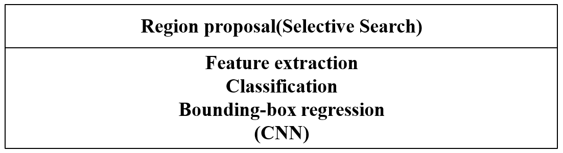
Two Fast R-CNN algorithm
-
One image generates 1K~2K candidate regions ( using the Selective Search method)
-
Input the image into the network to obtain the corresponding feature map , and project the candidate frame generated by the SS algorithm onto the feature map to obtain the corresponding feature matrix
-
Scale each feature matrix to a 7x7 feature map through the ROI pooling layer , and then flatten the feature map through a series of fully connected layers to get the prediction result
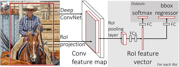
2.1 Calculate the entire image feature
Fast-RCNN sends the entire image into the network, and then extracts the corresponding candidate regions from the feature image. The features of these candidate regions do not need to be recalculated.
2.2 RoI Pooling Layer
RoI Pooling Layer (region of interest pooling layer) is a mechanism for extracting regions of interest from convolutional feature maps . RoI refers to the Region of Interest (region of interest), which refers to the bounding box obtained by the target detection algorithm in the input image.
The role of the RoI Pooling Layer is to map RoI regions of different sizes to outputs of the same size. Specifically, it first divides each RoI region into fixed-size sub-regions, and then performs a max-pooling operation on each sub-region to obtain a fixed-size output. The advantage of this is that it can ensure that RoI regions of different sizes can be processed, and map them to output feature maps of the same size, which is convenient for subsequent classification and regression tasks. does not limit the size of the input image
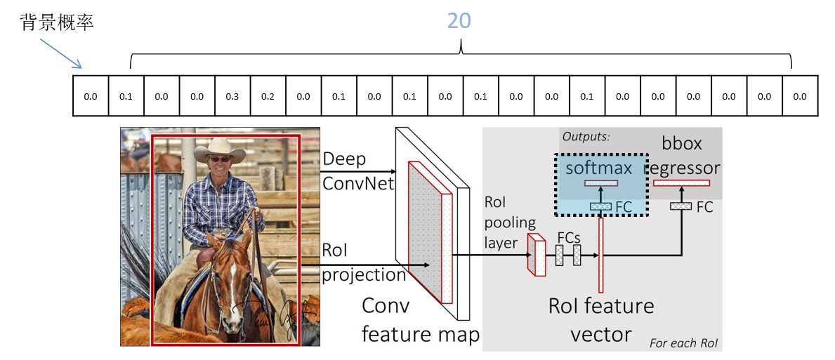
2.3 Classifier
Output the probability of N+1 categories (N is the type of detection target, 1 is the background) a total of N+1 nodes
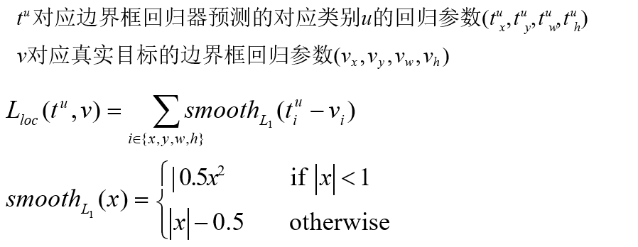
2.4 Bounding box regressor
Output the candidate bounding box regression parameters (dx, dy, dw, dh) corresponding to N+1 categories , a total of (N+1)x4 nodes
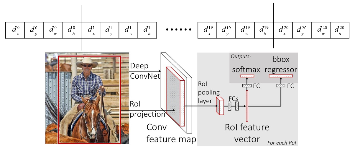
Bounding box regressor
Output the candidate bounding box regression parameters ( ) corresponding to N+1 categories , a total of (N+1)x4 nodes
They are the center x, y coordinates, and width and height of the candidate box respectively
Respectively for the final predicted bounding box center x, y coordinates, and width and height
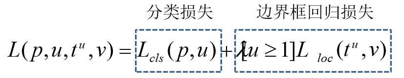
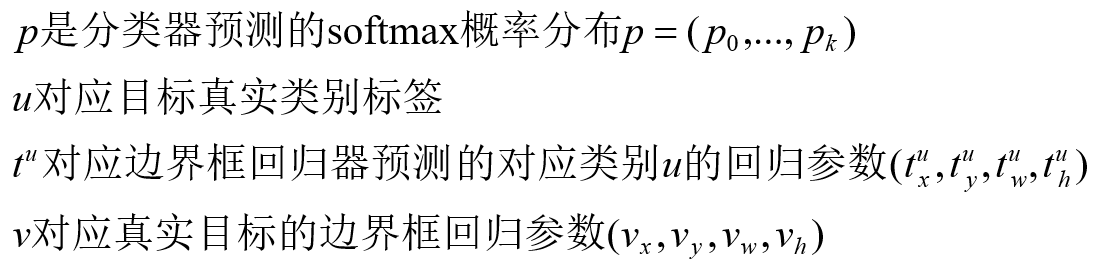
2.5 Multi-task loss
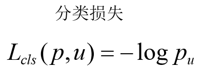
2.6 Cross Entropy Loss cross entropy loss
1. For multi-classification problems (softmax output, the sum of all output probabilities is 1)
![]()
2. For binary classification problems ( sigmoid output, each output node is irrelevant to each other)
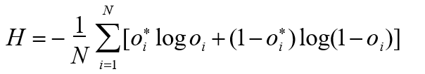
![]()
2.7 Fast R-CNN framework