Digital Image Processing and Its Applications Matlab- Fourier transform (with code)

1.Objectives:

1, two-dimensionally grasp the DFT and the physical significance
2, grasp the DFT dimensional MATLAB program
3, spatial filtering and frequency domain filtering

2.Experiment Content：

Learning to use functions fft2, ifft2, abs, angle, fftshift, imfilter, fspecial, freqz2; logarithmic display method;
achieve positive and negative Fourier transform, Gaussian low pass filtering and high pass filtering laplacian.

3.Experiment Principle:

See the book.

4.Experiment Steps Result and Conlusion：

1, using MATLAB digital Fourier transform image
is read and displayed in FIG Fig0316 (3) (third_from_top) .tif , dimensional FFT transform for F in the figure, to move the center of the spectrum of its DC component F1, calculating the real part RR, the imaginary part II, phase angle angle, calculated by the two methods and amplitude A1 = abs (F1) = sqrt and A2 (the RR. ^{2 + II.} 2), respectively, and show A1 A2, and compared.

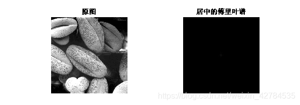
CON: from a first one of the chart, after Fourier transformation, the frequency range is mainly concentrated in the low frequency region, there can be seen a bright spot in the middle of the image, the remainder being black

CON: After logarithmic enhancement, you can see the details of the low-frequency component, we found two ways to find the amplitude spectrum obtained is somewhat different, but the overall layout is also roughly the same

2, the approximate impulse function dimensional Fourier transform

Impulse function A, as A two-dimensional Fourier transform of B, and B moves to DC component center of the spectrum B1, respectively, and mesh display imshow logarithmic function (log (1 + abs (B1 ) A mold and B1) )

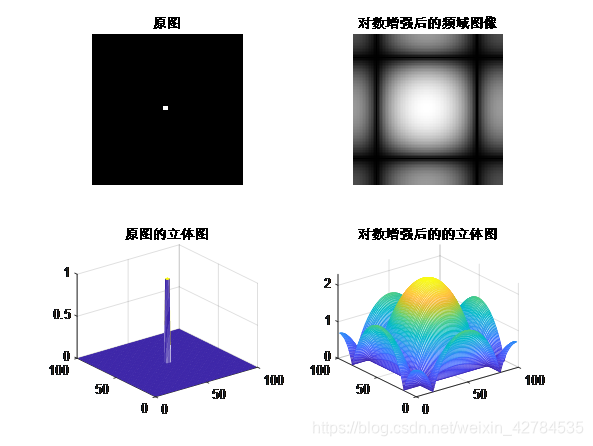
CON: left is generated similar impulse function, highlights the middle, surrounded by black right is its spectrum, it can be seen from the left, where most of the color area in FIG either white or black, substantially no change Therefore the low frequency component or the majority, where the transfer of black and white, color changes rapidly, therefore there will be some high frequency components, and therefore around the right, areas represent high-frequency components have bright spots.

CON: This is a perspective view of two drawn mesh, corresponding to the above two graphs, the FIG bright place on the amplitude of the high

3, spatial filtering and frequency domain filtering

FIG Fig0504 (a) (gaussian-noise) .ti (ff), respectively, and spatial frequency filtering.

Spatial filtering : generating fspecial 9 * 9, the standard deviation of the Gaussian filter w 2, of a function f IMFilter spatially filtered, to obtain a filtered image fi1.

Frequency domain filtering : The above-described Gaussian filter 256 * w which is obtained in the form of 256 W with a frequency-domain function freqz2, W used in the frequency domain filtered image f (note that the DC component in the center of the spectrum W), to give Ff,

Find its inverse Fourier transform (ifft2), to obtain a filtered image fi2 .

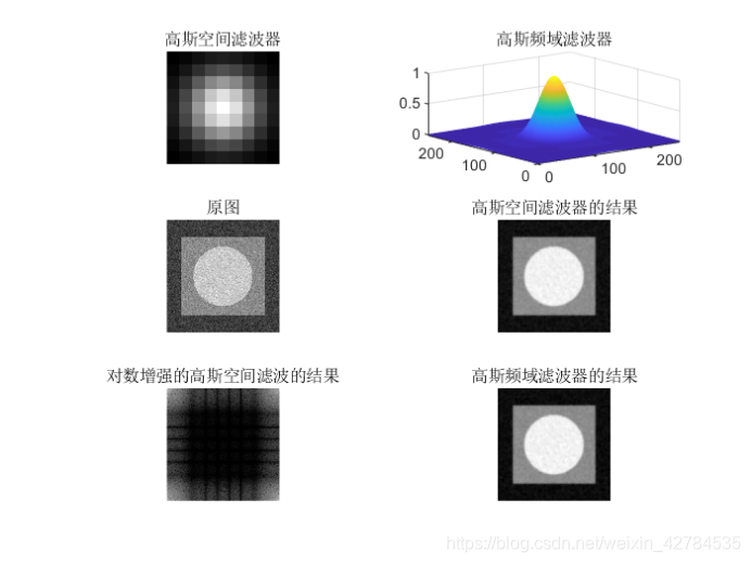
W imshow display a function, a display function W mesh, with the display module imshow f, fi1, Ff logarithmic, fi2.
Compare fi1 and fi2.

CON: FIG picture is noisy, can clearly be seen after filtering through filter effect

CON: top left is a time domain image of a spatial filter, top right is the frequency domain, it is mainly the low frequency filter. Bottom left is a filtered frequency spectrum after image, you can see a low frequency component (distributed around) the area to be brighter, larger values ​​representative, bottom right is filtered after FIG.

[Appendix] program

clear all;clc;
%第1题
f=imread('E:\数字图像处理\程序与图像\图像库\Fig0316(3)(third_from_top).tif');  %读取图像，获得信息
figure(1);
subplot(2,2,1);
imshow(f);%显示图像
title('原图');  

F=fft2(f);%傅里叶变换
subplot(2,2,2);
F1=fftshift(F);%居中
S=abs(F1);%居中的傅里叶谱
imshow(S, [])%显示图像
title('居中的傅里叶谱');     

RR=real(F1);%傅里叶谱的实部
II=imag(F1);%傅里叶谱的虚部
Angle=atan2(imag(F1),real(F1));%相角
A1=abs(F1);
A2=sqrt(RR.^2+II.^2);
subplot(2,2,3);
S1=log(1+A1);
imshow(S1, [])%显示图像
title('A1');
subplot(2,2,4);
S2=log(1+A2);
imshow(S2, [])%显示图像
title('A2');    
%第2题
A=zeros(99,99); 
A(49:51,49:51)=1;
B=fft2(A);
B1=fftshift(B);%居中
S1=log(1+abs(B1));%对数增强
S2=log(1+abs(A));%对数增强
figure(2); 
subplot(2,2,1);
imshow(A)%显示图像
title('原图');   
subplot(2,2,2);
imshow(S1, [])%显示图像
title('对数增强后的频域图像');
subplot(2,2,3);
mesh(A);
title('原图的立体图');
subplot(2,2,4);
mesh(S1);
title('对数增强后的的立体图');
%第3题
f=imread('E:\数字图像处理\程序与图像\图像库\Fig0504(a)(gaussian-noise).tif');  %读取图像，获得信息
w=fspecial('gaussian',[9 9],2);
fi1=imfilter(f,w,'replicate');  

W=freqz2(w,256,256);
W1=ifftshift(W);
F=fft2(f);
Ff=F.*W1;
fi2=ifft2(Ff);%fi2=uint8(fi2);
fi2=mat2gray(fi2); 

figure(3);
subplot(3,2,1);
imshow(w,[]);
title('高斯空间滤波器'); 

subplot(3,2,2);
mesh(W);
title('高斯频域滤波器'); 

subplot(3,2,3);
imshow(f);
title('原图'); 

subplot(3,2,4);
imshow(fi1,[]);
title('高斯空间滤波器的结果'); 

subplot(3,2,5);
imshow(log(1+abs(Ff)),[]);
title('对数增强的高斯空间滤波的结果'); 

subplot(3,2,6);
imshow(fi2);
title('高斯频域滤波器的结果');

[Image] is given above