深入理解“用于中文闲聊的GPT2模型”项目
- 论文部分提炼
- 1. Improving Language Understandingby Generative Pre-Training(GPT)
- 2. Language Models are Unsupervised Multitask Learners(GPT-2)
- 摘要
- 介绍
- 方法
- 实验
- Children’s Book Test(CBT)
- LAMBADA
- Winograd Schema Challenge
- Reading Comprehension
- Summarization
- Translation
- Question Answering
- Generalization vs Memorization
- 近期工作
- 结论
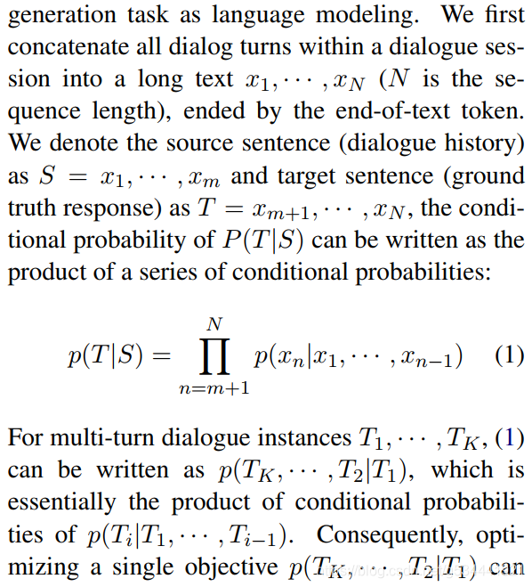
- 3. DIALOGPT : Large-Scale Generative Pre-trainingfor Conversational Response Generation
- 代码学习及调试
本文为对于GPT2 for Chinese chitchat项目的理解与学习
https://github.com/yangjianxin1/GPT2-chitchat
论文部分提炼
1. Improving Language Understandingby Generative Pre-Training(GPT)
摘要
自然语言理解包括一系列不同的任务,如文本蕴涵、问答、语义相似性评估和文档分类。尽管大型的未标记文本语料库非常丰富,但用于学习这些特定任务的标记数据却非常稀少,这使得对有偏向性的模型来说,要充分执行这些任务是一个挑战。与以前的方法相比,我们在微调期间使用任务感知的输入转换来实现有效的转换,同时要求对模型体系结构进行最小的更改。我们在一系列自然语言理解的基准上证明了我们的方法的有效性,我们的面向一般任务模型优于使用专门为每项任务设计体系结构的训练模型,在所研究的12项任务中,有9项显著提高了技术水平。
介绍
在自然语言处理(NLP)中,有效地从原始文本中学习是减轻对监督学习依赖的关键。
然而,由于两个主要原因,利用未标记文本中超过单词级别的信息是一个挑战。
首先,不清楚什么类型的优化目标在学习对传输有用的文本表示方面最有效。最近的研究着眼于不同的目标,如语言建模,机器翻译,语篇连贯,每一种方法在不同的任务上都优于其他方法。
第二,对于将这些学习到的表象传递给目标任务的最有效方式,目前还没有达成共识。
现有技术涉及将任务特定的更改与模型体系结构相结合。使用内部学习方案并添加辅助学习目标。这些不确定性使得开发有效的语言处理半监督学习方法变得非常困难。本文采用无监督预训练和监督微调相结合的方法,探讨了一种半监督的语言理解任务方法。我们的目标是学习一种普遍的表达方式,这种表达方式很少适应各种各样的任务。我们假设使用人工标注的训练示例(目标任务)访问一个大的未标记文本语料库和多个数据集。我们的设置不要求这些目标任务与未标记的语料库位于同一域中。
我们采用两阶段训练程序。首先,我们使用语言对未标记的数据进行建模,以学习神经网络模型的初始参数。随后,我们使用相应的有监督目标将这些参数应用于目标任务。
对于我们的模型架构,我们使用Transformer,它已经被证明在各种任务上都有很强的执行能力,比如机器翻译、文档生成和语法分析。与RNN等替代方案相比,这种模型选择为我们提供了一个更结构化的内存,用于处理文本中的长期依赖项,从而在各种任务中产生健壮的转换性能。 在转换过程中,我们使用从交叉样式( traversal-style)方法派生的特定于任务的输入自适应,该过程将结构化文本输入作为单个连续的令牌序列。正如我们在实验中所证明的,这些调整使我们能够有效地微调,对预先训练的模型的架构进行最小的更改。
最近工作
NLP的半监督学习
这种范式广泛应用于序列标记或文本分类,最早的方法是使用未标记的数据来计算单词级或短语级的统计信息,然后将其用作一个监督模型中的特征。在过去的几年里,研究人员已经证明了使用单词嵌入,即在未标记的语料库上进行训练,来提高任务的平均性能。然而,这些方法主要是传递单词级的信息,而我们的目标是获取更高级别的语义。
最近的方法已经研究了从未标记的数据中学习和使用超过单词级别的语义,短语级或句子级的嵌入,可以使用未标记的语料库进行训练,已经被用来将文本编码成适合各种目标任务的向量表示。
无监督预训练
无监督预训练是半监督学习的一种特殊情况,其目的是寻找一个好的初始点,而不是修改监督学习目标。早期的工作探索了该技术在图像分类和分类任务中的应用,随后的研究表明,预训练可以作为一种正则化方案,使深层神经网络具有更好的泛化能力。在最近的工作中,该方法被用来帮助训练深度神经网络完成各种任务,如图像分类、语音识别、实体消歧和机器翻译。
最接近我们的工作是使用目标语言对神经网络进行预训练,然后在有人监督的情况下对其进行微调。然而,尽管预训练阶段有助于捕获一些语言信息,但它们对LSTM模型的使用将其可预测性限制在较短的范围内。与此相反,我们选择的 Transformer网络允许我们捕获更长范围的语言结构,这在我们的实验中得到了证明。此外,我们还展示了我们的模型在更广泛的任务上的有效性,包括自然语言推理、释义和故事完成。其他方法使用预先训练语言或机器翻译模型的隐藏表示作为辅助特征,同时训练目标模型的监督模型。这涉及到每个目标分离的任务的大量新参数,而在传输期间,我们需要对模型体系结构进行最小的更改。
辅助训练目标
增加辅助无监督训练目标是半监督学习的另一种形式。Collobert和Weston的早期工作使用了各种各样的辅助NLP任务,如词性标注、分块、命名实体识别和语言模型化来改进语义角色标注,在目标任务目标上添加一个辅助语言模型,并展示了序列标记任务的性能增益。我们的实验也使用一个辅助的目标,但是正如我们所展示的,无监督的预训练已经学习了与目标任务相关的几个语言方面。
框架
我们的训练程序分为两个阶段。第一阶段是在一个大的文本语料库上学习一个高容量的语言模型。接下来是一个微调阶段,在这个阶段中,我们将模型调整为带有标记数据的判别任务。
无监督预训练
给定一个无监督语料库的标记S= {u1,…,un},我们使用一个标准的语言模型来最大化以下可能性
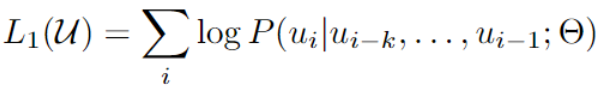
其中,k是上下文窗口的大小,P为使用参数Θ的神经网络建模的条件概率型。这些参数是用随机梯度下降训练的。
在我们的实验中,我们使用多层Transformer解码器[34]作为语言模型,它是Transformer的变体,此模型对输入上下文标记应用多头自注意操作,然后是位置前馈层,以生成分布在目标标记上的输出:
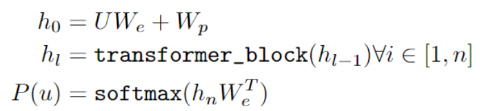
其中U是令牌的上下文向量,n是层数,We是令牌嵌入矩阵,Wp是位置嵌入矩阵。
监督预训练
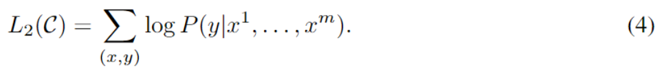
在用公式1中的目标模型训练后,我们将参数调整到有监督的目标任务。我们假设一个带标签的数据集C,其中每个实例由一系列输入标记x1,…,xm和标签y组成。输入通过我们预先训练的模型来获得最终Transformer组的激活hml,然后将其输入一个参数为Wy的加线性输出层(added linear output layer)来预测y:

最大化以下目标:
我们还发现,包括语言建模作为辅助目标的微调有益于:
- 改进监督模式的泛化
- 加速收敛
具体来说,我们优化了以下目标(权重λ):

总的来说,在微调期间,我们只需要Wy和定界符(delimiter tokens)的嵌入。
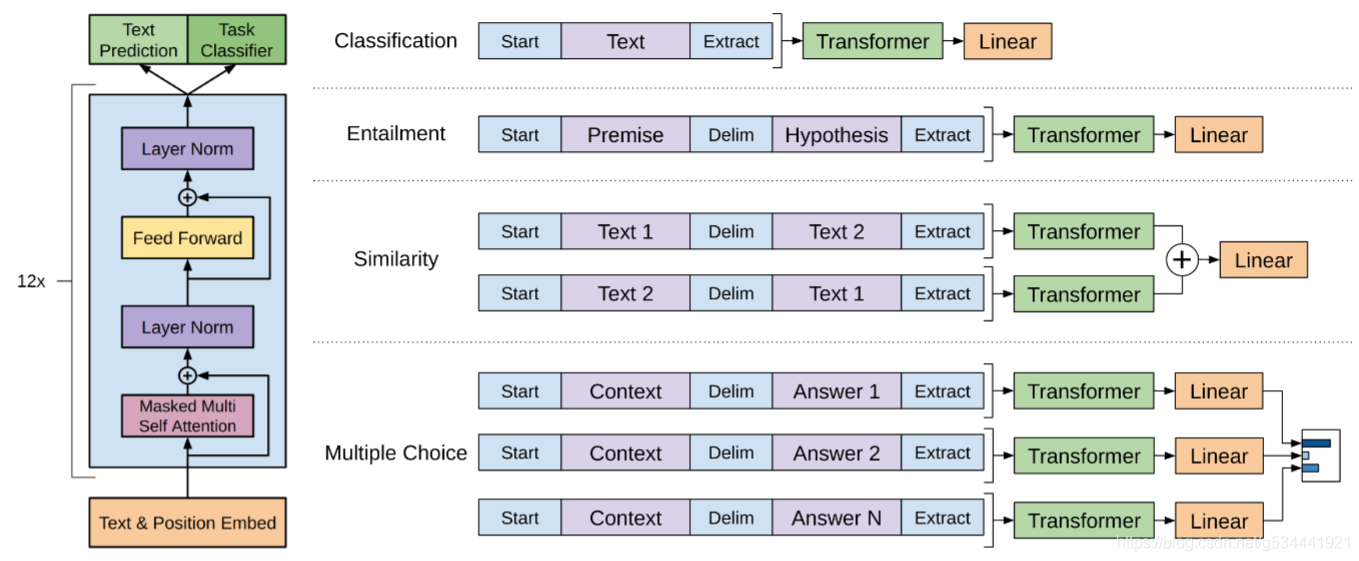
左:这项工作中使用的Transformer 结构和训练目标。
右:用于对不同任务进行微调的输入转换。
我们将所有结构化输入转换为令牌序列,然后由我们的预训练模型进行处理,之后是 linear+softmax layer。
特定任务的输入转换
对于一些任务,如文本分类,我们可以直接微调我们的模型,如上所述。
某些其他任务,如问答或文本蕴涵,具有结构化输入,如顺序句子对或文档、问题和答案的三元组当然也可以。由于我们的预训练模型是在连续的文本序列上训练的,因此我们需要进行一些修改才能将其应用于这些任务。
先前的工作提出了基于转换表示的任务特定的学习体系结构。
这种方法重新引入了大量特定于任务的定制,并且没有对这些额外的体系结构组件使用迁移学习。相反,我们使用遍历样式(traversal-style)方法,将结构化输入转换为我们的预训练模型可以处理的有序序列即将结构化输入转换为一个有序序列。这些输入转换允许我们避免跨任务对架构进行大量更改。我们在下面简要描述了这些输入转换,图1提供了一个直观的说明。所有转换都包括添加随机初始化的开始和结束标记(〈s〉,〈e〉)。
文字蕴涵(Textual entailment)
对于蕴涵任务,我们将 premise p和 hypothesis h与分隔符token($)连接起来。
相似性
对于相似性任务,两个被比较的句子没有内在的顺序。为了反映这一点,我们修改输入序列以包含两个可能的句子顺序(中间有分隔符)并分别处理产生两个序列表示hml,在被馈入线性输出层之前按元素添加。
问答与常识推理
对于这些任务,我们会得到一个context document z, a question q ,和一组可能的答案{ak}。我们将文档上下文和问题与每个可能的答案连接起来,在两者之间添加一个分隔符标记以获取[z;q;$;ak]。这些序列中的每一个都是用我们的模型独立处理的,然后通过一个softmax对其进行规范化,从而在可能的答案上产生一个输出分布。
2. Language Models are Unsupervised Multitask Learners(GPT-2)
摘要
自然语言处理任务如问答,机器翻译,阅读理解,阅读理解和总结是典型的在特定任务的数据集上进行的监督学习。我们证明了当语言模型在由数以百万计的网页组成名为WebText的新数据集上进行训练时,可以无需监督学习这些任务。
在文档+问题的条件下,由语言模型生成的回答在CoQA数据集上达到了55的F1—在没有使用127000多个训练示例的情况下匹配或超过了四分之三的基线系统的性能。
语言模型的容量对于zero-shot task transfer的成功和增加它对 log-linear fashion across task任务的性能是必不可少的。
GPT-2是一个1.5B参数的Transformer ,zero-shot的条件下在7/8个语言模型的测试数据集上做到了state of the art,但对WebText依旧欠拟合。
启示:建立从自然发生的演示(naturally occurring demonstrations)中学习解决任务的语言处理系统。
介绍
机器学习系统在有大数据集高容量模型的情况下在特定任务上表现良好,但脆弱且对数据分布十分敏感。我们转向更通用的系统,无需手动打标签(无监督)。
方法
由于监督目标与无监督目标相同,但仅在序列的子集上进行评估,无监督目标的全局最小值也就是监督目标的全局最小值(忽略关于密度估计的一个原则性训练目标 the concerns with density estimationas a principled training objective discussed in (Sutskeveret al., 2015) are side stepped.)。
虽然对话是一种很好的文本数据,但是它的限制比较大,我们的方法鼓励建立尽可能大且多样的数据集,以便在尽可能多的领域和上下文中收集任务的自然语言演示(demonstrations )。(简单说,什么类型的文本都可以达到学习语义信息的效果。)
输入表示
通用语言模型(LM)应该能够计算(并生成)任何字符串的概率。
当前大规模LMs包括预处理步骤,如lower-casing, tokenization, 和out-of-vocabulary tokens,这些步骤限制了可建模字符串的空间。当前字节级LMs在大型数据集(如十亿字基准)上与字级LMs不具有竞争性。(两者在表现上相差不大)
字节对编码(BPE)是字符和单词级语言建模之间的一个折中(practical middle ground),它有效地在频繁符号序列的单词级输入和不频繁符号序列的字符级输入之间进行插值。尽管名称不同,reference BPE实现通常操作Unicode代码点,而不是字节序列。这些实现需要包含Unicode符号的全部空间,以便对所有Unicode字符串建模。这将导致在添加任何multi-symbol tokens之前,基本词汇表超过130000。与BPE通常使用的32000到64000个token vocabularies相比,这是一个令人望而却步的大问题。相反,字节级版本的BPE只需要256大小的基本词汇表。然而,直接将BPE应用于字节序列会导致次优合并(sub-optimal merges),因为BPE使用贪心的基于频率的启发式(greedy frequency based heuristic)算法来构建令牌词汇表。我们观察到BPE包括许多常见词的版本,比如dog,因为它们出现在许多变体中比如dog. dog!dog?这将导致有限词汇槽和模型容量(limitedvocabulary slots and model capacity)的次优分配。为了避免这种情况,我们防止BPE为任意字节序列跨字符类别合并。我们为空格添加了一个例外,这显著地提高了压缩效率,同时在多个vocab tokens之间添加了最小的单词碎片。
这种输入表示允许我们结合词级LMs的经验优势和字节级方法的通用性。因为我们的方法可以为任何Unicode字符串分配一个概率,这允许我们在任何数据集上评估LMs,而不管预处理、标记或vocab大小如何。
模型
我们的LMs使用基于Transformer 的架构。该模型在很大程度上遵循了OpenAI GPT模型的细节的基础上做了一定改动。
- Layer normalization被移到了每个子块的输入,类似于pre-activation residual networkk (He et al., 2016)。并在最后一个自我注意块之后添加额外的layer normalization。
- 修改初始化方法,用模型深度计算剩余路径上的累积量(accountsfor the accumulation on the residual path with model depthis used)。我们将初始化时剩余层的权重按1/√n的系数进行缩放,其中是剩余层的数量。
- 词汇量扩大到50257。我们还可以将上下文大小从512增加到1024个tokens ,并使用更大的batch size 512。
实验
语言建模数据集上的结果通常以平均负对数概率规范预测单元(the average negative log probability per canonical prediction unit)比例缩放或指数化(scaled or exponentiated)的量,通常是一个字符、一个字节或一个单词。我们根据一个WebText LM计算一个数据集的对数概率(log-probability),然后除以规范单元( canonical units)的数量,来评估相同的数量。对于这些数据集中的许多,WebText LMs将在分布之外进行显著的测试,必须积极地预测标准化的文本(standardized text)、标记化工件(tokenization artifacts),如断开的标点和收缩(disconnected punctuationand contractions)、无序的句子,甚至是UNK,而这在WebText中极少-在400亿字节内仅发生26次。由于这些去标记器(de-tokenizers)是可逆的,我们仍然可以计算一个数据集的对数概率(log probability ),它们可以被看作是一种简单的域适应形式(domain adaptation)。我们观察到带有去标记器的GPT-2有着2.5到5的perplexity 的增益。
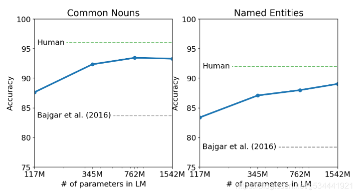
Children’s Book Test(CBT)
儿童书籍测试(CBT)(Hill等人,2015)旨在研究LMs在不同类别词汇(命名实体、名词、动词和介词)上的表现。CBT不是报告perplexity而是报告自动构造完形填空测试的accuracy ,其中任务是预测一个省略单词的10个可能选项中的哪一个是正确的。
LAMBADA
LAMBADA数据集(Paperno等人,2016年)测试了系统在文本中建立长期依赖关系模型的能力。任务是预测句子的最后一个单词,人类至少需要50个上下文标记才能成功预测。
GPT-2将the state of the art从99.8(Graves et al,2016)提升到8.6的perplexity ,并使LMs在该测试中的准确性从19%(DeHghani等人,2018)提高到52.66%。对GPT-2错误的调查表明,大多数预测是句子的有效延续,但不是预设的最后一个单词。这表明LM没有使用额外的有用约束,即单词必须是句子的结尾。添加一个停止字过滤器(stop-word filter)作为一个近似值,进一步将精度提高到63.24%,提高了本任务的总体状态4%。
Winograd Schema Challenge
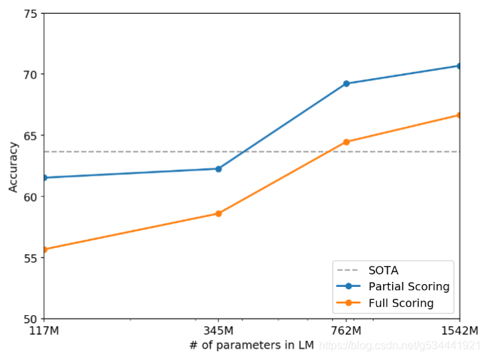
Winograd Schema challenge(Levesque等人,2012)的构建是为了通过测量系统解决文本中歧义的能力来衡量系统执行常识推理的能力。
Reading Comprehension
会话问答数据集(CoQA)Reddy等人。(2018)由来自7个不同领域问答者之间的自然语言对话的一系列文件组成。CoQA测试阅读理解能力和模型回答依赖于历史会话的能力。
似乎表现不好,作者甩锅给了无监督。
Summarization
经常关注文章的最新内容,或者把具体细节搞混,比如有多少辆车卷入车祸,或者帽子或衬衫上有什么标志。接近基线水平,仅略优于从文章中选择3个随机句子。
Translation
在WMT-14英语-法语测试集上,GPT-2获得了5的BLEU,这比以前的无监督词翻译中的双语词典逐字替换略差(Conneau 等人., 2017b)。在WMT-14法语-英语测试集上,GPT-2能够利用其非常强大的英语语言模型来显著提高性能,达到11.5 BLEU。这优于(Artetxe et al.,2017)和(Lampleet al.,2017)中的几个无监督机器翻译基线,但仍比当前最佳无监督机器翻译方法(Artetxe et al.,2019)的33.5 BLEU差得多。作者对此也感到十分诧异,因为语料库中的噪音并不多(英文数据中的法语内容不到500分之一)。
Question Answering
测试语言模型中包含哪些信息的一个潜在方法是评估是不是经常产生问题的仿真陈述式的回答(factoid-style,不真实但可以使人信以为真)。
GPT-2在回答常用于阅读理解的数据集如SQUAD时回答的正确率为4.1%。作为比较,最小的模型不超过一个非常简单的基线的1.0%的精确度,该基线为每种问题类型(谁、什么、在哪里等)返回最常见的答案。GPT-2能正确回答5.3倍以上的问题,表明模型容量是导致神经网络系统在这类任务中表现不佳的主要因素。GPT-2分配给其生成的应答器的概率经过了很好的校准,GPT-2对其最有信心的1%的问题的准确率为63.1%。GPT-2的性能仍然比开放域问答系统的30%到50%的范围差很多,这些系统混合了信息检索和抽取文档问答。(Alberti 等人., 2019).
Generalization vs Memorization
计算机视觉领域的最新研究表明,常见的图像数据集包含大量的近似重复的图像。例如,CIFAR-10在训练图像和测试图像之间有3.3%的重叠(Barz&Denzler,2019)。这导致了对机器学习系统泛化性能的过度报道。随着数据集大小的增加,这个问题变得越来越可能,这表明类似的现象可能发生在WebText上,因此,分析有多少测试数据也出现在训练数据中是很重要的。
为了研究这个问题,我们创建了包含8-grams of WebText training set token的Bloom筛选器。
我们的方法优化了召回,虽然手动检查重叠显示了许多常见的短语,但由于重复的数据,还有许多更长的匹配。
令人担忧的是,这样的问题普遍存在。但从结果上讲,排除这种干扰所带来的的准确率下降并没有太严重的影响(在排除任何重叠的所有实例时重新计算度量结果perplexity从8.6 到了 8.7,并将精度从63.2%降低到62.9%。)
目前,我们建议使用基于n-gram重叠的重复数据消除作为一个重要的验证步骤,并在为新的NLP数据集创建训练和测试拆分时进行健全性检查。
判断WebText LMs 的表现是否归因于记忆的另一种可能的方法是在他们自己的留出集(held-out set)上检查他们的表现。WebText的训练集和测试集的性能相似,并且随着模型大小的增加而共同提高。这表明即使是GPT-2在很多方面仍然对WebText欠拟合。
近期工作
这项工作的很大一部分衡量了在较大数据集上训练的较大语言模型的性能。
我们计划对诸如 decaNLP 和GLUE等基准进行微调,尤其是因为目前还不清楚GPT-2的额外的训练数据和能力是否足以克服BERT所描述的单向表示的低效性。
结论
当一个大型语言模型在一个足够大和多样化的数据集上训练时,它能够在多个领域和数据集上表现良好。在zero-shot setting下模型能够执行的任务多样性表明,高容量模型被训练以最大限度地增加足够多的文本语料库的可能性,开始学习如何执行惊人数量的任务,而不需要明确的监督。
3. DIALOGPT : Large-Scale Generative Pre-trainingfor Conversational Response Generation
摘要
DIALOGPT是在2005~2017的Reddit评论链中提取的147M个对话上进行训练的,扩展了Hugging Face PyTorch Transformer ,使其在单轮对话的自动评估和人工评估方面都达到了接近人类表现的性能。生成了比baseline systems更高相关性、丰富度和上下文一致性的回复。
介绍
OpenAI的GPT-2表明:在非常大的数据集上训练的Transformer 模型可以捕获文本数据中的长期依赖关系,并生成流畅、词汇多样和内容丰富的文本。这样的模型有能力捕捉具有细粒度的文本数据,并产生高分辨率的输出,从而更好地模仿人类编写的真实文本。
自然语言回复生成是文本生成的一个子类别,目标都是生成与提示句相关的更自然的文本。
但是,模拟对话的独特挑战在于,人类对话包含了两个参与者可能相互竞争的目标(encapsulates the possibly competing goals of two participants),本质上更多样化。因此,与其他文本生成任务(如NMT神经网络机器翻译,文本总结等)相比,一对多问题(one-to-many problem)更大。而一般来说,人类的对话也比较非正式、嘈杂,而且,当以文本聊天的形式出现时,往往包含非正式的缩写或句法/词汇错误。
大多数开放域回复生成系统都存在内容或样式不一致。缺乏长期的语境信息,以及回复过于平淡(安全回复)的问题。虽然这些问题可以通过专门为提高信息内容而设计的建模策略来缓解,但基于Transformer 的结构,如GPT-2,使用多层自注意力机制,采用全连接对跨越注意力(allow fully-connected cross-attention to the full context)进行高效计算来关注整个上下文,似乎是探索更一般解决方案的自然选择。
Transformer 模型可以更好地保存长期依赖信息,从而提高内容的一致性。同时也因为深层结构有着更大的模型容量,可以比RNN模型更好地利用大规模数据集。
与GPT-2的对比
- 相同点:DIALOGPT也是一个自回归语言模型,采用多层Transformer 作为模型体系结构…
- 不同点:是对在从Reddit评论链中提取的大规模对话对/会话上进行训练的。作者推测这样可以更好地获取P(Target,Source)在具有更细粒度的对话流中的联合分布(This should enable DIALOGPT to capturethe joint distribution of P(Target,Source) in conversational flow with finer granularity)。
数据集
Reddit评论可以自然地扩展为树结构的回复链,因为回复一个线程的线程形成了后续线程的根节点。我们将每条路径从根节点提取到叶节点,作为包含多轮对话的训练实例。
对以下情形进行过滤:
- 对话中存在URL
- 含有三个以上的单词重复
- 如果回复中不包含至少一个 top-50最频繁使用的英语单词(eg., “the”, “of”, “a”),这代表着可能不是一个英文句子
- 回复包含特殊标记,如“[”或“]”,因为这可能是标记语言。
- 提问或回复超过200个单词
- 存在黑名单中的敏感词
方法
模型结构
在采用通用Transformer 结构的GPT-2架构上利用堆叠的masked多头自注意层来训练大量的网络文本数据。
Tricks
- layer normalization
- 根据我们改进的模型深度计算的初始化方案(a initialization scheme that accounts
for model depth that we modified) - 字节对编码(byte pairencodings)
将多轮对话转链接为长文本形式

互信息最大化
计算maximum mutual information (MMI) 来应对生成的回复信息量低的问题。
采用一个预训练的反向模型来从给定的答句预测出问句P(Source|target)。先使用top-K采样来生成一系列假设,然后再利用**P(Source|Hypothesis)**来对假设进行重排,以此来惩罚安全回复。
这里我的理解是:对于不同的问题,可能可以进行相同的安全回复。比如
我们一起去看电影好不好?
我们一起去爬山好不好?
......
等等类似的句子,完全可以用简单的 好的。 这个回复来对应,这时给出这个回复的概率就会很高。
但是如果我们用**P(Source|Hypothesis)**来重排的话就会发现
好呀,我最喜欢看电影了!
这种回复的情况下对应 我们一起去看电影好不好? 的可能性就会高的多,这样回复就会更倾向于可能包含对应于问句更多的信息的假设。
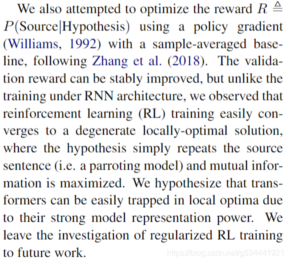
关于强化学习的尝试
简单讲:容易陷入局部最优,表现为答句简单重复问句。
训练加速
- 懒加载数据降低读取频率。
- 采用分离的异步数据进程来扩展训练。(We also leverage separate asynchronous data processes to scale the training. )
- 进一步采用了一种动态批处理策略,将长度相似的对话分组到同一批中,从而提高了训练吞吐量。
DSTC-7 Dialogue Generation Challenge
DSTC (Dialog System Technology Challenges) 一个端到端的对话建模任务,目标是通过注入基于外部知识的信息来生成会话回答,从而超越闲聊。
(the goal is to generate conversation responses that go beyond chitchat by injecting information that is grounded in external knowledge. )此任务与通常认为的目标导向、任务导向或完成任务(goal-oriented, task-oriented, or task-completion)的对话不同,因为没有特定或预定义的目标。相反,它的目标是人与人之间的相互作用,在这种相互作用中,潜在的目标通常是不明确或事先未知的。
关于自动测试分数高于人类的解释
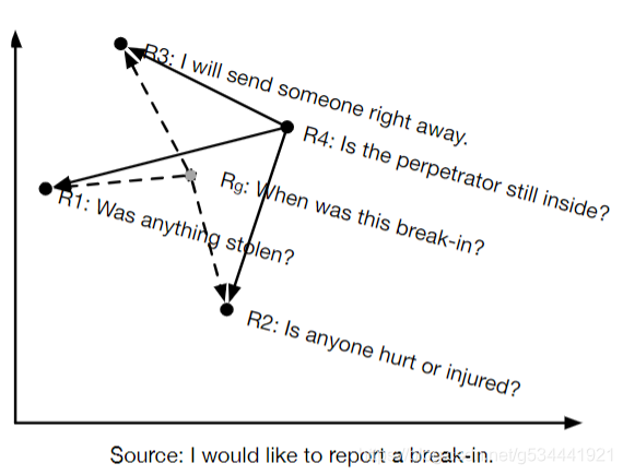
如:假设R1-R4是可能的人类问答,R1-R3是我们用来做测试的“真实回答”,那么在语义空间里,一个训练好的模型生成的回答Rg,将很可能靠近所有可能回复的几何中心,而这个几何中心(Rg)到参考点(R3)的距离可能小于R4到R3的距离。这就使得在自动测试分数上,模型表现超越了人类。
另外,人类评审甚至有时也给了MMI高于人类回复的分数,因为人类回复可能更加的不稳定和特殊化,或者带有评审们不熟悉的网络用语。
局限与挑战
主要还是隐性的敏感语句,包括历史,性别等方面的冒犯。
结论
发布了开放域的预训练模型DIALOGPT。
代码学习及调试
灰色注释看起来太难受了,注释我用//意思一下。
项目结构
- config:存放GPT2模型的参数的配置文件
- data
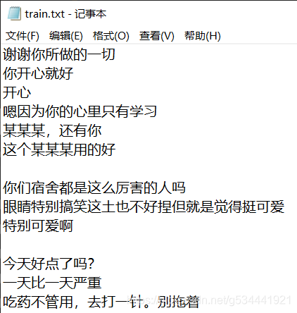
- train.txt:默认的原始训练集文件,存放闲聊语料
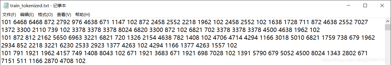
- train_tokenized.txt:对原始训练语料进行顺序tokenize之后的文件,用于dialogue model的训练
- train_mmi_tokenized.txt:对原始训练语料进行逆序tokenize之后的文件,用于mmi model的训练
- dialogue_model:存放对话生成的模型
- mmi_model:存放MMI模型(maximum mutual information scoring function),
用于预测P(Source|response) - sample:存放人机闲聊生成的历史聊天记录
- vocabulary:存放GPT2模型的字典
- train.py:训练代码
- interact.py:人机交互代码
train.py
//定义填充
PAD = '[PAD]'
pad_id = 0
logger = None
主要功能模块汇总
def setup_train_args():
    """
    设置训练参数
    """
def set_random_seed(args):
    """
    设置训练的随机种子
    """
def create_logger(args):
    """
    将日志输出到日志文件和控制台
    """
def create_model(args, vocab_size):
    """

    :param args:
    :param vocab_size:字典大小
    :return:
    """
def preprocess_raw_data(args, tokenizer, n_ctx):
    """
    对原始语料进行处理,将原始语料转换为用于train的token id,对于每个dialogue,将其处于成如下形式"[CLS]utterance1[SEP]utterance2[SEP]utterance3[SEP]"
    :param args:
    :param tokenizer:
    :param n_ctx:GPT2模型的上下文窗口大小,对于超过n_ctx(n_ctx包括了特殊字符)的dialogue进行截断
    :return:
    """
def calculate_loss_and_accuracy(outputs, labels, device):
    """
    计算非pad_id的平均loss和准确率
    :param outputs:
    :param labels:
    :param device:
    :return:
    """
def collate_fn(batch):
    """
    计算该batch中的所有sample的最长的input,并且将其他input的长度向其对齐
    :param batch:
    :return:
    """
def train(model, device, train_list, multi_gpu, args):
def evaluate(model, device, test_list, multi_gpu, args):
setup_train_args()
def setup_train_args():
    """
    设置训练参数
    """
这里对parser.add_argument做下对于与项目相关的解释,节省一点检索时间。
class ArgumentParser(_AttributeHolder, _ActionsContainer):
    """Object for parsing command line strings into Python objects.

    Keyword Arguments:
        - prog -- The name of the program (default: sys.argv[0])
        - usage -- A usage message (default: auto-generated from arguments)
        - description -- A description of what the program does
        - epilog -- Text following the argument descriptions
        - parents -- Parsers whose arguments should be copied into this one
        - formatter_class -- HelpFormatter class for printing help messages
        - prefix_chars -- Characters that prefix optional arguments
        - fromfile_prefix_chars -- Characters that prefix files containing
            additional arguments
        - argument_default -- The default value for all arguments
        - conflict_handler -- String indicating how to handle conflicts
        - add_help -- Add a -h/-help option
        - allow_abbrev -- Allow long options to be abbreviated unambiguously
    """

    def __init__(self,
                 prog=None,
                 usage=None,
                 description=None,
                 epilog=None,
                 parents=[],
                 formatter_class=HelpFormatter,
                 prefix_chars='-',
                 fromfile_prefix_chars=None,
                 argument_default=None,
                 conflict_handler='error',
                 add_help=True,
                 allow_abbrev=True):
- prog - 程序的名称(默认:sys.argv[0])
- usage - 描述程序用途的字符串(默认值:从添加到解析器的参数生成)
- description - 在参数帮助文档之前显示的文本(默认值:无)
- epilog - 在参数帮助文档之后显示的文本(默认值:无)
- parents - 一个 ArgumentParser 对象的列表,它们的参数也应包含在内
- formatter_class - 用于自定义帮助文档输出格式的类
- prefix_chars - 可选参数的前缀字符集合(默认值:’-’)
- fromfile_prefix_chars - 当需要从文件中读取其他参数时,用于标识文件名的前缀字符集合(默认值:None)
- argument_default - 参数的全局默认值(默认值: None)
- conflict_handler - 解决冲突选项的策略(通常是不必要的)
- add_help - 为解析器添加一个 -h/–help 选项(默认值: True)
- allow_abbrev - 如果缩写是无歧义的,则允许缩写长选项 (默认值:True)
接一下来用项目中的实例具体过一下:
parser.add_argument('--device', default='0,1', type=str, required=False, help='设置使用哪些显卡'
- 第一项 ‘–device’ 代表程序名称
- default=‘0,1’ 代表在执行python脚本时如果对 ‘–device’ 项不进行设置时默认输入的值
- type=str 输入的类型为字符串
- required=False 通常,argparse模块假定 -f 和 --bar 等标志表示可选参数,这些参数在命令行中总是可以忽略的。要使选项成为必需的,可以为要添加的required=keyword参数指定True。这里是False则表明这项参数非必须。
- help=‘设置使用哪些显卡’,用户在执行脚本时输入-h时对相应参数显示的帮助信息。
parser.add_argument('--no_cuda', action='store_true', help='不使用GPU进行训练')
- action=‘store_true’
ArgumentParser 对象将命令行参数与动作相关联。这些动作可以做与它们相关联的命令行参数的任何事,尽管大多数动作只是简单的向 parse_args() 返回的对象上添加属性。action 命名参数指定了这个命令行参数应当如何处理。
‘store_true’ and ‘store_false’ - 这些是 ‘store_const’ 分别用作存储 True 和 False 值的特殊用例。另外,它们的默认值分别为 False 和 True。这里自然是True喽,与设置default和type的组合功能类似,适用场景有所差别。
相关参数作者注释写得极尽清楚,这里不再赘述。
set_random_seed()
torch.backends.cudnn.benchmark
pytorch基础—cudnn.benchmark和cudnn.deterministic以及如何禁用cudnn
def set_random_seed(args):
    """
    设置训练的随机种子
    """
	//为各种类型的随机值设置相同的种子
    torch.manual_seed(args.seed)
    random.seed(args.seed)
    np.random.seed(args.seed)
    //cuda相关设置
    if args.cuda:
        torch.backends.cudnn.deterministic = True
        torch.backends.cudnn.benchmark = False
- torch.backends.cudnn.deterministic = True 将这个 flag 置为 True 的话,每次返回的卷积算法将是确定的,即默认算法。如果配合上设置 Torch 的随机种子为固定值的话,应该可以保证每次运行网络的时候相同输入的输出是固定的。用以保证实验的可重复性。
- torch.backends.cudnn.benchmark 设置这个 flag 可以让内置的 cuDNN 的 auto-tuner 自动寻找最适合当前配置的高效算法,来达到优化运行效率的问题。这里关闭了该选项。
- 如果网络的输入数据维度或类型上变化不大,设置 torch.backends.cudnn.benchmark = true
可以增加运行效率; - 如果网络的输入数据在每次 iteration 都变化的话,会导致 cnDNN 每次都会去寻找一遍最优配置,这样反而会降低运行效率。
- 如果网络的输入数据维度或类型上变化不大,设置 torch.backends.cudnn.benchmark = true
create_logger()
打印日志部分与功能实现无关,有兴趣的朋友可以自行了解。
create_model()
注释很详细,具体细节遇到再看。
preprocess_raw_data()
if "\r\n" in data:
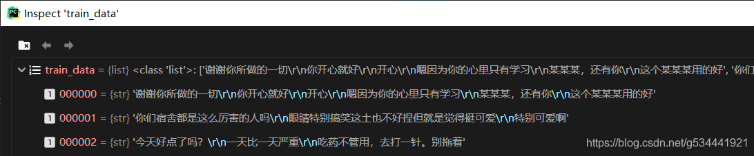
train_data = data.split("\r\n\r\n")
else:
train_data = data.split("\n\n")
Python ‘\r’, ‘\n’, ‘\r\n’ 的彻底理解
将语料库对话分段存入train_data

with open(args.train_tokenized_path, "w", encoding="utf-8") as f:
for dialogue_index, dialogue in enumerate(tqdm(train_data)):
if "\r\n" in data:
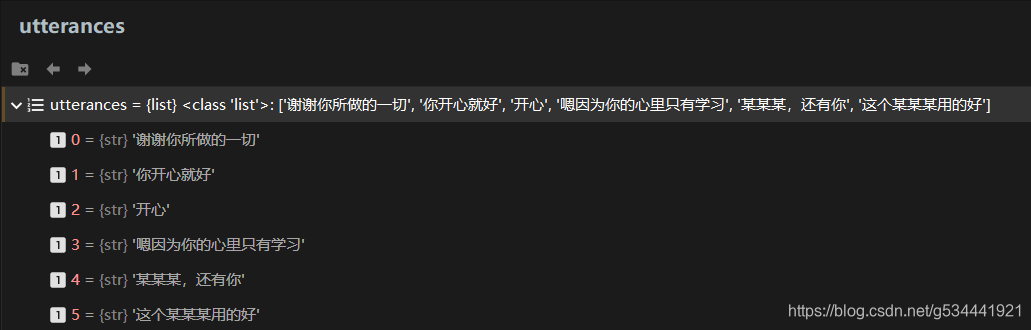
utterances = dialogue.split("\r\n")
else:
utterances = dialogue.split("\n")
dialogue_ids = [tokenizer.cls_token_id] # 每个dialogue以[CLS]开头
for utterance in utterances:
dialogue_ids.extend([tokenizer.convert_tokens_to_ids(word) for word in utterance])
dialogue_ids.append(tokenizer.sep_token_id) # 每个utterance之后添加[SEP],表示utterance结束
# 对超过n_ctx的长度进行截断,否则GPT2模型会报错
dialogue_ids = dialogue_ids[:n_ctx]
for dialogue_id in dialogue_ids:
f.write(str(dialogue_id) + ' ')
# 最后一条记录不添加换行符
if dialogue_index < len(train_data) - 1:
f.write("\n")
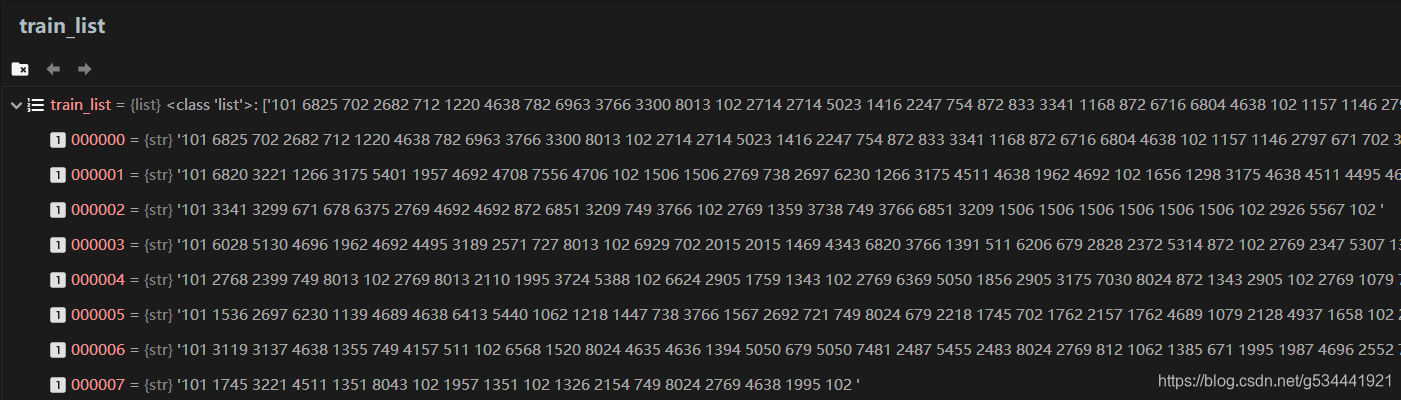
这部分很好理解,放几张图辅助一下。
一次循环:
101代表CLS,102代表SEP。
dialogue_ids<class 'list'>: [101, 6468, 6468, 872, 2792, 976, 4638, 671, 1147, 102, 872, 2458, 2552, 2218, 1962, 102, 2458, 2552, 102, 1638, 1728, 711, 872, 4638, 2552, 7027, 1372, 3300, 2110, 739, 102, 3378, 3378, 3378, 8024, 6820, 3300, 872, 102, 6821, 702, 3378, 3378, 3378, 4500, 4638, 1962, 102]
tqdm是很好用的进度条工具,感兴趣的可以自行研究细节。
preprocess_mmi_raw_data()
def preprocess_mmi_raw_data(args, tokenizer, n_ctx):
    """
    对原始语料进行处理,将原始语料的每段对话进行翻转,然后转换为用于train MMI模型的token id,对于每个dialogue,将其处于成如下形式"[CLS]utterance N[SEP]utterance N-1[SEP]utterance N-2[SEP]"
    :param args:
    :param tokenizer:
    :param n_ctx:GPT2模型的上下文窗口大小,对于超过n_ctx(n_ctx包括了特殊字符)的dialogue进行截断
    :return:
    """
		dialogue_ids = [tokenizer.cls_token_id]  # 每个dialogue以[CLS]开头
        for utterance in reversed(utterances):  # 将一段对话进行翻转
            dialogue_ids.extend([tokenizer.convert_tokens_to_ids(word) for word in utterance])
            dialogue_ids.append(tokenizer.sep_token_id)  # 每个utterance之后添加[SEP],表示utterance结束
<class 'list'>: [101, 6821, 702, 3378, 3378, 3378, 4500, 4638, 1962, 102, 3378, 3378, 3378, 8024, 6820, 3300, 872, 102, 1638, 1728, 711, 872, 4638, 2552, 7027, 1372, 3300, 2110, 739, 102, 2458, 2552, 102, 872, 2458, 2552, 2218, 1962, 102, 6468, 6468, 872, 2792, 976, 4638, 671, 1147, 102]
这里做了什么呢,其实是将某一段对话的顺序做了下颠倒。简单讲:
普通: CLS 句1 SEP 句2 SEP 句3 SEP
MMI: CLS 句3 SEP 句2 SEP 句1 SEP
单句内语序不变。
训练流程(可以先从这里看起,遇到问题再Ctrl+F定位对应模块)
训练普通对话模型
- git clone 该项目
- 下载50w中文闲聊语料,将train.txt放在项目目录的data文件夹下
- 根据需要修改参数设置的default值
- 我们首先生成对话模型(无MMI)
我采用的是修改默认值直接运行的方式,故action设为’store_true’时,直接运行会是False,因为并没有激活参数。
所以本次以这两项的状态如下:
rser.add_argument('--raw', action='store_false', help='是否对原始训练语料做tokenize。若尚未对原始训练语料进行tokenize,则指定该参数')
parser.add_argument('--train_mmi', action='store_true', help="若指定该参数,则训练DialoGPT的MMI模型")
调试过程中,我们会进入部分子函数,此时我会用0~n序号来表示第n层子函数,避免思路丢失,那么先从0 main开始
0 main
def main():
    args = setup_train_args()
    # 日志同时输出到文件和console
    global logger
    logger = create_logger(args)
    # 当用户使用GPU,并且GPU可用时
    args.cuda = torch.cuda.is_available() and not args.no_cuda
    device = 'cuda' if args.cuda else 'cpu'
    logger.info('using device:{}'.format(device))
    # 为CPU设置种子用于生成随机数,以使得结果是确定的
    # 为当前GPU设置随机种子;如果使用多个GPU,应该使用torch.cuda.manual_seed_all()为所有的GPU设置种子。
    # 当得到比较好的结果时我们通常希望这个结果是可以复现
    if args.seed:
        set_random_seed(args)

    # 设置使用哪些显卡进行训练
    os.environ["CUDA_VISIBLE_DEVICES"] = args.device
    # 初始化tokenizer
    tokenizer = BertTokenizer(vocab_file=args.vocab_path)
    # tokenizer的字典大小
    vocab_size = len(tokenizer)

    global pad_id
    pad_id = tokenizer.convert_tokens_to_ids(PAD)

    # 创建对话模型的输出目录
    if not os.path.exists(args.dialogue_model_output_path):
        os.mkdir(args.dialogue_model_output_path)
这部分注释已经很清楚了。
    # 加载GPT2模型
    model, n_ctx = create_model(args, vocab_size)
0 main -> 1 create_model()
    if args.pretrained_model:  # 如果指定了预训练的GPT2模型
        model = GPT2LMHeadModel.from_pretrained(args.pretrained_model)
    else:  # 若没有指定预训练模型,则初始化模型
        model_config = transformers.modeling_gpt2.GPT2Config.from_json_file(args.model_config)
        model = GPT2LMHeadModel(config=model_config)
    # 根据tokenizer的vocabulary调整GPT2模型的voca的大小
    model.resize_token_embeddings(vocab_size)
我们这次没有指定预训练的GPT2模型,则从josn文件中获取模型设置。
model_config = transformers.modeling_gpt2.GPT2Config.from_json_file(args.model_config)
model_config_dialogue_small.json
{
  "initializer_range": 0.02,
  "layer_norm_epsilon": 1e-05,
  "n_ctx": 300,
  "n_embd": 768,
  "n_head": 12,
  "n_layer": 10,
  "n_positions": 300,
  "vocab_size": 13317
}
model_config补全了一些默认项。
{
  "attn_pdrop": 0.1,
  "embd_pdrop": 0.1,
  "finetuning_task": null,
  "initializer_range": 0.02,
  "layer_norm_epsilon": 1e-05,
  "n_ctx": 300,
  "n_embd": 768,
  "n_head": 12,
  "n_layer": 10,
  "n_positions": 300,
  "num_labels": 1,
  "output_attentions": false,
  "output_hidden_states": false,
  "output_past": true,
  "pruned_heads": {},
  "resid_pdrop": 0.1,
  "summary_activation": null,
  "summary_first_dropout": 0.1,
  "summary_proj_to_labels": true,
  "summary_type": "cls_index",
  "summary_use_proj": true,
  "torchscript": false,
  "use_bfloat16": false,
  "vocab_size": 13317
}
model = GPT2LMHeadModel(config=model_config)
1 create_model() -> 2 GPT2LMHeadModel
GPT2LMHeadModel
GPT2模型transformer ,顶部有语言模型头(language modeling head)(权重与输入嵌入绑定的线性层)。
class GPT2LMHeadModel(GPT2PreTrainedModel):
def __init__(self, config):
super(GPT2LMHeadModel, self).__init__(config)
self.transformer = GPT2Model(config)
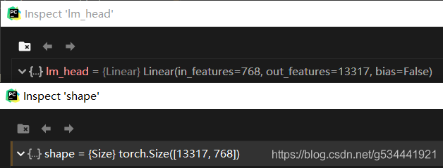
self.lm_head = nn.Linear(config.n_embd, config.vocab_size, bias=False)
self.init_weights()
self.tie_weights()
这里Transformer我们就先不跟进了,后边再另行记录。
lm_head自然就是语言模型头了。
2 GPT2LMHeadModel -> 3 init_weights
    def init_weights(self):
        """ Initialize and prunes weights if needed. """
        # Initialize weights
        self.apply(self._init_weights)
这里递归调用 _init_weights 函数对所有的子项(源码中的submodule / .children())进行权重初始化。
module
GPT2Model(
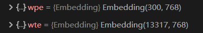
(wte): Embedding(13317, 768)
(wpe): Embedding(300, 768)
(drop): Dropout(p=0.1, inplace=False)
(h): ModuleList(
(0): Block(
(ln_1): LayerNorm((768,), eps=1e-05, elementwise_affine=True)
(attn): Attention(
(c_attn): Conv1D()
(c_proj): Conv1D()
(attn_dropout): Dropout(p=0.1, inplace=False)
(resid_dropout): Dropout(p=0.1, inplace=False)
)
(ln_2): LayerNorm((768,), eps=1e-05, elementwise_affine=True)
(mlp): MLP(
(c_fc): Conv1D()
(c_proj): Conv1D()
(dropout): Dropout(p=0.1, inplace=False)
)
)
(1): Block(
(ln_1): LayerNorm((768,), eps=1e-05, elementwise_affine=True)
(attn): Attention(
(c_attn): Conv1D()
(c_proj): Conv1D()
(attn_dropout): Dropout(p=0.1, inplace=False)
(resid_dropout): Dropout(p=0.1, inplace=False)
)
(ln_2): LayerNorm((768,), eps=1e-05, elementwise_affine=True)
(mlp): MLP(
(c_fc): Conv1D()
(c_proj): Conv1D()
(dropout): Dropout(p=0.1, inplace=False)
)
)
(2): Block(
(ln_1): LayerNorm((768,), eps=1e-05, elementwise_affine=True)
(attn): Attention(
(c_attn): Conv1D()
(c_proj): Conv1D()
(attn_dropout): Dropout(p=0.1, inplace=False)
(resid_dropout): Dropout(p=0.1, inplace=False)
)
(ln_2): LayerNorm((768,), eps=1e-05, elementwise_affine=True)
(mlp): MLP(
(c_fc): Conv1D()
(c_proj): Conv1D()
(dropout): Dropout(p=0.1, inplace=False)
)
)
(3): Block(
(ln_1): LayerNorm((768,), eps=1e-05, elementwise_affine=True)
(attn): Attention(
(c_attn): Conv1D()
(c_proj): Conv1D()
(attn_dropout): Dropout(p=0.1, inplace=False)
(resid_dropout): Dropout(p=0.1, inplace=False)
)
(ln_2): LayerNorm((768,), eps=1e-05, elementwise_affine=True)
(mlp): MLP(
(c_fc): Conv1D()
(c_proj): Conv1D()
(dropout): Dropout(p=0.1, inplace=False)
)
)
(4): Block(
(ln_1): LayerNorm((768,), eps=1e-05, elementwise_affine=True)
(attn): Attention(
(c_attn): Conv1D()
(c_proj): Conv1D()
(attn_dropout): Dropout(p=0.1, inplace=False)
(resid_dropout): Dropout(p=0.1, inplace=False)
)
(ln_2): LayerNorm((768,), eps=1e-05, elementwise_affine=True)
(mlp): MLP(
(c_fc): Conv1D()
(c_proj): Conv1D()
(dropout): Dropout(p=0.1, inplace=False)
)
)
(5): Block(
(ln_1): LayerNorm((768,), eps=1e-05, elementwise_affine=True)
(attn): Attention(
(c_attn): Conv1D()
(c_proj): Conv1D()
(attn_dropout): Dropout(p=0.1, inplace=False)
(resid_dropout): Dropout(p=0.1, inplace=False)
)
(ln_2): LayerNorm((768,), eps=1e-05, elementwise_affine=True)
(mlp): MLP(
(c_fc): Conv1D()
(c_proj): Conv1D()
(dropout): Dropout(p=0.1, inplace=False)
)
)
(6): Block(
(ln_1): LayerNorm((768,), eps=1e-05, elementwise_affine=True)
(attn): Attention(
(c_attn): Conv1D()
(c_proj): Conv1D()
(attn_dropout): Dropout(p=0.1, inplace=False)
(resid_dropout): Dropout(p=0.1, inplace=False)
)
(ln_2): LayerNorm((768,), eps=1e-05, elementwise_affine=True)
(mlp): MLP(
(c_fc): Conv1D()
(c_proj): Conv1D()
(dropout): Dropout(p=0.1, inplace=False)
)
)
(7): Block(
(ln_1): LayerNorm((768,), eps=1e-05, elementwise_affine=True)
(attn): Attention(
(c_attn): Conv1D()
(c_proj): Conv1D()
(attn_dropout): Dropout(p=0.1, inplace=False)
(resid_dropout): Dropout(p=0.1, inplace=False)
)
(ln_2): LayerNorm((768,), eps=1e-05, elementwise_affine=True)
(mlp): MLP(
(c_fc): Conv1D()
(c_proj): Conv1D()
(dropout): Dropout(p=0.1, inplace=False)
)
)
(8): Block(
(ln_1): LayerNorm((768,), eps=1e-05, elementwise_affine=True)
(attn): Attention(
(c_attn): Conv1D()
(c_proj): Conv1D()
(attn_dropout): Dropout(p=0.1, inplace=False)
(resid_dropout): Dropout(p=0.1, inplace=False)
)
(ln_2): LayerNorm((768,), eps=1e-05, elementwise_affine=True)
(mlp): MLP(
(c_fc): Conv1D()
(c_proj): Conv1D()
(dropout): Dropout(p=0.1, inplace=False)
)
)
(9): Block(
(ln_1): LayerNorm((768,), eps=1e-05, elementwise_affine=True)
(attn): Attention(
(c_attn): Conv1D()
(c_proj): Conv1D()
(attn_dropout): Dropout(p=0.1, inplace=False)
(resid_dropout): Dropout(p=0.1, inplace=False)
)
(ln_2): LayerNorm((768,), eps=1e-05, elementwise_affine=True)
(mlp): MLP(
(c_fc): Conv1D()
(c_proj): Conv1D()
(dropout): Dropout(p=0.1, inplace=False)
)
)
)
(ln_f): LayerNorm((768,), eps=1e-05, elementwise_affine=True)
)
    def _init_weights(self, module):
        """ Initialize the weights.
        """
        //判断是否是(nn.Linear, nn.Embedding, Conv1D)类型中的一个
        if isinstance(module, (nn.Linear, nn.Embedding, Conv1D)):
            # Slightly different from the TF version which uses truncated_normal for initialization
            # cf https://github.com/pytorch/pytorch/pull/5617
            // @1
            module.weight.data.normal_(mean=0.0, std=self.config.initializer_range)
            if isinstance(module, (nn.Linear, Conv1D)) and module.bias is not None:
            	// @2
                module.bias.data.zero_()
        elif isinstance(module, nn.LayerNorm):
        	// @3
            module.bias.data.zero_()
            module.weight.data.fill_(1.0)
@1
torch.nn.init.normal_(tensor, mean=0.0, std=1.0)
对所有的Embedding,Linear,Conv1D的weight值使用从正态分布
中提取的值填充输入张量。
@2
对Linear,Conv1D存在bias的项的偏置(bias)值置0。
@3
对LayerNorm偏置置0,权重赋1。
2 GPT2LMHeadModel <- 3 init_weights
2 GPT2LMHeadModel -> 3 tie_weights
    def tie_weights(self):
        """ Make sure we are sharing the input and output embeddings.
            Export to TorchScript can't handle parameter sharing so we are cloning them instead.
        """
        self._tie_or_clone_weights(self.lm_head,
                                   self.transformer.wte)
将lm_head和transformer.wte进行参数共享。
1 create_model() <- 2 GPT2LMHeadModel
1 create_model() -> 2 resize_token_embeddings
model.resize_token_embeddings(vocab_size)
如果new_num_tokens != config.vocab_size,则对模型的input token embeddings 矩阵进行resize 。
如果模型类有一个“tie_weights()”方法,请在之后注意绑定权重嵌入。
		base_model = getattr(self, self.base_model_prefix, self)  // 获取模型
        model_embeds = base_model._resize_token_embeddings(new_num_tokens)
        if new_num_tokens is None:
            return model_embeds

        // 更新vocab_size
        self.config.vocab_size = new_num_tokens
        base_model.vocab_size = new_num_tokens

        // 如果需要则重新设置参数共享
        if hasattr(self, 'tie_weights'):
            self.tie_weights()

        return model_embeds
base_model = getattr(self, self.base_model_prefix, self)
获取模型

1 create_model() <- 2 resize_token_embeddings
0 main <-1 create_model()
model.to(device)
Pytorch to(device)
将所有最开始读取数据时的tensor变量copy一份到device所指定的GPU上去,之后的运算都在GPU上进行。
    # 对原始数据进行预处理,将原始语料转换成对应的token_id
    if args.raw and args.train_mmi:  # 如果当前是要训练MMI模型
        preprocess_mmi_raw_data(args, tokenizer, n_ctx)
    elif args.raw and not args.train_mmi:  # 如果当前是要训练对话生成模型
        preprocess_raw_data(args, tokenizer, n_ctx)
本次调试我们采用 preprocess_raw_data,细节见上方(Ctrl+F查找)
(preprocess_raw_data函数只需完整运行一次,对原始数据进行预处理,将原始语料转换成对应的token_id后即保存在train_tokenized.txt,之后只需改变预设参数–raw的预设状态即可不必重复执行此步骤)。
    # 是否使用多块GPU进行并行运算
    multi_gpu = False
    if args.cuda and torch.cuda.device_count() > 1:
        logger.info("Let's use GPUs to train")
        model = DataParallel(model, device_ids=[int(i) for i in args.device.split(',')])
        multi_gpu = True
    # 记录模型参数数量
    num_parameters = 0
    parameters = model.parameters()
    for parameter in parameters:
        num_parameters += parameter.numel()
    # 加载数据
    logger.info("loading traing data")
    if args.train_mmi:  # 如果是训练MMI模型
        with open(args.train_mmi_tokenized_path, "r", encoding="utf8") as f:
            data = f.read()
    else:  # 如果是训练对话生成模型
        with open(args.train_tokenized_path, "r", encoding="utf8") as f:
            data = f.read()
    data_list = data.split("\n")
    // 分训练集和测试集
    train_list, test_list = train_test_split(data_list, test_size=0.2, random_state=1)
0 main -> 1 train()
    train_dataset = MyDataset(train_list)
    train_dataloader = DataLoader(train_dataset, batch_size=args.batch_size, shuffle=True, num_workers=args.num_workers,
                                  collate_fn=collate_fn)
pytorch数据加载方法。按batch_size乱序调用train_list。
torch.utils.data.DataLoader
collate_fn (callable, optional) – merges a list of samples to form a mini-batch of Tensor(s). Used when using batched loading from a map-style dataset.
1 train() -> 2 model.train()
model.train()
    def train(self, mode=True):
        self.training = mode
        for module in self.children():
            module.train(mode)
        return self
对每个子模型进行训练。


2 model.train() -> 3 module.train(mode)


。。。。。。。
        self.training = mode   // mode的值为True
        for module in self.children():
            module.train(mode)
        return self
这部分只是将模型的每个部分的training标识置为true。
2 model.train() <- 3 module.train(mode)
1 train() <- 2 model.train()
    # 计算所有epoch进行参数优化的总步数total_steps
    total_steps = int(train_dataset.__len__() * args.epochs / args.batch_size / args.gradient_accumulation)
    # 设置优化器,并且在初始训练时,使用warmup策略
    optimizer = transformers.AdamW(model.parameters(), lr=args.lr, correct_bias=True)
    scheduler = transformers.WarmupLinearSchedule(optimizer, warmup_steps=args.warmup_steps, t_total=total_steps)
gradient_accumulation,optimizer 先不作详解。
WarmupLinearSchedule
用于动态调整训练速率,加快训练。
class WarmupLinearSchedule(LambdaLR):
    """ Linear warmup and then linear decay.
        Linearly increases learning rate from 0 to 1 over `warmup_steps` training steps.
        Linearly decreases learning rate from 1. to 0. over remaining `t_total - warmup_steps` steps.
    """
    def __init__(self, optimizer, warmup_steps, t_total, last_epoch=-1):
        self.warmup_steps = warmup_steps
        self.t_total = t_total
        super(WarmupLinearSchedule, self).__init__(optimizer, self.lr_lambda, last_epoch=last_epoch)

    def lr_lambda(self, step):
        if step < self.warmup_steps:
            return float(step) / float(max(1, self.warmup_steps))
        return max(0.0, float(self.t_total - step) / float(max(1.0, self.t_total - self.warmup_steps)))
    # 用于统计每次梯度累计的loss
    running_loss = 0
    # 统计一共训练了多少个step
    overall_step = 0
    # 记录tensorboardX
    tb_writer = SummaryWriter(log_dir=args.writer_dir)
    # 记录 out of memory的次数
    oom_time = 0
    # 开始训练
    for epoch in range(args.epochs):
        epoch_start_time = datetime.now()
        for batch_idx, input_ids in enumerate(train_dataloader):
            # 注意:GPT2模型的forward()函数,是对于给定的context,生成一个token,而不是生成一串token
            # GPT2Model的输入为n个token_id时,输出也是n个hidden_state,使用第n个hidden_state预测第n+1个token
            input_ids = input_ids.to(device)
            # 解决在运行过程中,由于显存不足产生的cuda out of memory的问题
本次调试batchsize=8, 0为PAD。
input_ids,shape=(8,133)
tensor([[ 101, 2582,  720,  ...,    0,    0,    0],
        [ 101, 3800, 2692,  ...,    0,    0,    0],
        [ 101, 1638, 1638,  ...,    0,    0,    0],
        ...,
        [ 101, 1962, 2626,  ...,    0,    0,    0],
        [ 101, 1928, 1355,  ...,    0,    0,    0],
        [ 101, 1724, 2398,  ...,    0,    0,    0]])
            try:
                outputs = model.forward(input_ids=input_ids)
                loss, accuracy = calculate_loss_and_accuracy(outputs, labels=input_ids, device=device)
真正的训练开始了!
1 train() -> 2 model.forward(input_ids=input_ids)
outputs = model.forward(input_ids=input_ids)
    def forward(self, input_ids, past=None, attention_mask=None, token_type_ids=None, position_ids=None, head_mask=None,
                labels=None):
        transformer_outputs = self.transformer(input_ids,
                                               past=past,
                                               attention_mask=attention_mask,
                                               token_type_ids=token_type_ids,
                                               position_ids=position_ids,
                                               head_mask=head_mask)
        hidden_states = transformer_outputs[0]

        lm_logits = self.lm_head(hidden_states)

        outputs = (lm_logits,) + transformer_outputs[1:]
        if labels is not None:  //本次调试不涉及该条件
            # Shift so that tokens < n predict n
            shift_logits = lm_logits[..., :-1, :].contiguous()
            shift_labels = labels[..., 1:].contiguous()
            # Flatten the tokens
            loss_fct = CrossEntropyLoss(ignore_index=-1)
            loss = loss_fct(shift_logits.view(-1, shift_logits.size(-1)),
                            shift_labels.view(-1))
            outputs = (loss,) + outputs

        return outputs  # (loss), lm_logits, presents, (all hidden_states), (attentions)
        transformer_outputs = self.transformer(input_ids,
                                               past=past,
                                               attention_mask=attention_mask,
                                               token_type_ids=token_type_ids,
                                               position_ids=position_ids,
                                               head_mask=head_mask)
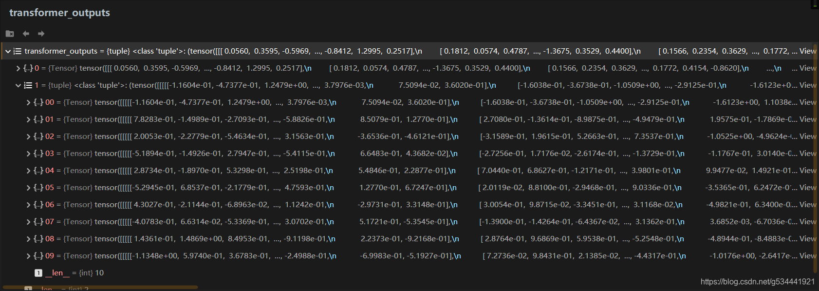
这部分其实是在transformer中进行前向计算获取相应输出。
关于transformer之后我会再详尽地总结一篇博客。这里我们跳过这个部分的解读。
我们只需关注transformer_outputs 的shape:
torch.Size([8, 133, 768]) 8为batchsize,133为该序列最大长度,768为预设Embedding长度。
hidden_states = transformer_outputs[0]
可以看到transformer_outputs[0]对应的是hidden_states
lm_logits = self.lm_head(hidden_states)
这里就是经过一个全连接层,没错,就是Transformer后面接个普通的全连接层。。。
记录下 lm_logits 的 shape: torch.Size([8, 133, 13317])
outputs = (lm_logits,) + transformer_outputs[1:]
这里是将transformer_outputs[0]换成了lm_logits,即用新的计算结果替换了之前的hidden state,再赋给outputs 。
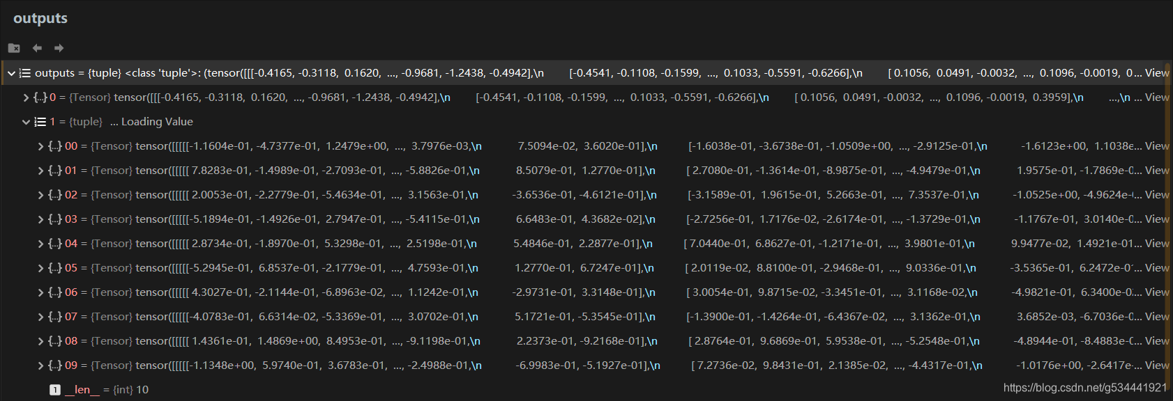
return outputs # (loss), lm_logits, presents, (all hidden_states), (attentions)
1 train() <- 2 model.forward(input_ids=input_ids)
loss, accuracy = calculate_loss_and_accuracy(outputs, labels=input_ids, device=device)
1 train() ->2 calculate_loss_and_accuracy()
def calculate_loss_and_accuracy(outputs, labels, device):
    """
    计算非pad_id的平均loss和准确率
    :param outputs:
    :param labels:
    :param device:
    :return:
    """
    logits = outputs[0]  # 每个token用来预测下一个token的prediction_score,维度:[batch_size,token_len,voca_size]
    # 用前n-1个token,预测出第n个token
    # 用第i个token的prediction_score用来预测第i+1个token。
    # 假定有input有n个token,则shift_logits表示model中第[0,n-2]个token的prediction_score,shift_labels表示第[1,n-1]的label
    shift_logits = logits[..., :-1, :].contiguous()
    shift_labels = labels[..., 1:].contiguous().to(device)

    loss_fct = CrossEntropyLoss(ignore_index=pad_id, reduction='sum')  # 忽略pad_id的loss,并对所有的非pad_id的loss进行求和
    loss = loss_fct(shift_logits.view(-1, shift_logits.size(-1)),
                    shift_labels.view(-1))

    _, preds = shift_logits.max(dim=-1)  # preds表示对应的prediction_score预测出的token在voca中的id。维度为[batch_size,token_len]

    # 对非pad_id的token的loss进行求平均,且计算出预测的准确率
    not_ignore = shift_labels.ne(pad_id)  # 进行非运算,返回一个tensor,若targets_view的第i个位置为pad_id,则置为0,否则为1
    num_targets = not_ignore.long().sum().item()  # 计算target中的非pad_id的数量

    correct = (shift_labels == preds) & not_ignore  # 计算model预测正确的token的个数,排除pad的tokne
    correct = correct.float().sum()

    accuracy = correct / num_targets
    loss = loss / num_targets
    return loss, accuracy
pytorch中contiguous()1
pytorch中contiguous()2
CrossEntropyLoss
shape:
shift_logits  torch.Size([8, 132, 13317])
shift_labels  torch.Size([8, 132])

shift_logits.view(-1, shift_logits.size(-1))  torch.Size([1056, 13317])
shift_labels.view(-1) torch.Size([1056])
1 train() <- 2 calculate_loss_and_accuracy()
_, preds = shift_logits.max(dim=-1) # preds表示对应的prediction_score预测出的token在vocab中的id。维度为[batch_size,token_len]
shift_logits.max(dim=-1):
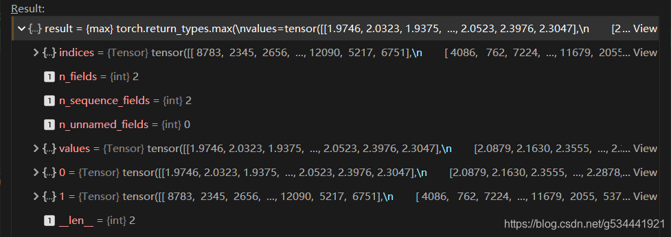
preds torch.Size([8, 132])
    # 对非pad_id的token的loss进行求平均,且计算出预测的准确率
    not_ignore = shift_labels.ne(pad_id)  # 进行非运算,返回一个tensor,若targets_view的第i个位置为pad_id,则置为0,否则为1
    num_targets = not_ignore.long().sum().item()  # 计算target中的非pad_id的数量

    correct = (shift_labels == preds) & not_ignore  # 计算model预测正确的token的个数,排除pad的tokne
    correct = correct.float().sum()

    accuracy = correct / num_targets
    loss = loss / num_targets
    return loss, accuracy
torch.ne(input, other, out=None) → Tensor
long() → Tensor
self.long() is equivalent to self.to(torch.int64).

item() → number
Returns the value of this tensor as a standard Python number. This only works for tensors with one element. For other cases, see tolist().

This operation is not differentiable.

Example:

>>> x = torch.tensor([1.0])
>>> x.item()
1.0
loss.backward() //反向传播就不解释了吧
		# 梯度裁剪解决的是梯度消失或爆炸的问题,即设定阈值
		torch.nn.utils.clip_grad_norm_(model.parameters(), args.max_grad_norm)
torch.nn.utils.clip_grad_norm_(parameters, max_norm, norm_type=2)
Clips gradient norm of an iterable of parameters.
The norm is computed over all gradients together, as if they were concatenated into a single vector. Gradients are modified in-place.
		# 进行一定step的梯度累计之后,更新参数
        if (batch_idx + 1) % args.gradient_accumulation == 0:
        running_loss += loss.item()
        # 更新参数
        optimizer.step()
        # 清空梯度信息
        optimizer.zero_grad()
        # 进行warm up
        scheduler.step()
        overall_step += 1
            except RuntimeError as exception:
                if "out of memory" in str(exception):
                    oom_time += 1
                    logger.info("WARNING: ran out of memory,times: {}".format(oom_time))
                    if hasattr(torch.cuda, 'empty_cache'):
                        torch.cuda.empty_cache()
                else:
                    logger.info(str(exception))
                    raise exception
        logger.info('saving model for epoch {}'.format(epoch + 1))
内存溢出检测及记录。
        logger.info('saving model for epoch {}'.format(epoch + 1))
        if args.train_mmi:  # 当前训练MMI模型
            model_path = join(args.mmi_model_output_path, 'model_epoch{}'.format(epoch + 1))
        else:  # 当前训练对话模型
            model_path = join(args.dialogue_model_output_path, 'model_epoch{}'.format(epoch + 1))
        if not os.path.exists(model_path):
            os.mkdir(model_path)
        model_to_save = model.module if hasattr(model, 'module') else model
        model_to_save.save_pretrained(model_path)
        logger.info('epoch {} finished'.format(epoch + 1))
        epoch_finish_time = datetime.now()
        logger.info('time for one epoch: {}'.format(epoch_finish_time - epoch_start_time))
模型保存及日志记录。
0 main <- 1 train()
0 main <- 1 evaluate()
def evaluate(model, device, test_list, multi_gpu, args):
    logger.info("start evaluating model")
    model.eval()
    logger.info('starting evaluating')
    # 记录tensorboardX
    tb_writer = SummaryWriter(log_dir=args.writer_dir)
    test_dataset = MyDataset(test_list)
    test_dataloader = DataLoader(test_dataset, batch_size=args.batch_size, shuffle=True, num_workers=args.num_workers,
                                 collate_fn=collate_fn)
    with torch.no_grad():
        for batch_idx, input_ids in enumerate(test_dataloader):
            input_ids.to(device)
            outputs = model.forward(input_ids=input_ids)
            loss, accuracy = calculate_loss_and_accuracy(outputs, labels=input_ids, device=device)

            if multi_gpu:
                loss = loss.mean()
                accuracy = accuracy.mean()
            if args.gradient_accumulation > 1:
                loss = loss / args.gradient_accumulation
                accuracy = accuracy / args.gradient_accumulation
            logger.info("evaluate batch {} ,loss {} ,accuracy {}".format(batch_idx, loss, accuracy))
            # tb_writer.add_scalar('loss', loss.item(), overall_step)
        logger.info("finishing evaluating")
loss, accuracy = calculate_loss_and_accuracy(outputs, labels=input_ids, device=device)
这里是通过直接计算输出(答句)和输入(问句)的交叉熵来评估,一般来讲应该是预测答句和预设答句做交叉熵的,不过鉴于对话生成的特殊性,这样的做法也无不可吧。
训练MMI对话模型
大部分是完全相同的,这里只讲变化。
0 main -> 1 preprocess_mmi_raw_data()
    if args.raw and args.train_mmi:  # 如果当前是要训练MMI模型
        preprocess_mmi_raw_data(args, tokenizer, n_ctx)
这部分请转至之前主要模块汇总的对应部分。
是的,这就是在训练过程中唯一的区别了。
普通对话生成(interact.py)
非核心部分就不重复讲解了,我们来看主要流程。
    history = []
    print('开始和chatbot聊天,输入CTRL + Z以退出')
    while True:
        try:
            text = input("user:")
            if args.save_samples_path:
                samples_file.write("user:{}\n".format(text))
            history.append(tokenizer.encode(text))
            input_ids = [tokenizer.cls_token_id]  # 每个input以[CLS]为开头
            for history_id, history_utr in enumerate(history[-args.max_history_len:]):
                input_ids.extend(history_utr)
                input_ids.append(tokenizer.sep_token_id)
            curr_input_tensor = torch.tensor(input_ids).long().to(device)
这里即输入一段字符串并在其头部加上CLS,结尾加SEP,并将序列转换为Tensor。
            generated = []
            # 最多生成max_len个token
            for _ in range(args.max_len):
                outputs = model(input_ids=curr_input_tensor)
                next_token_logits = outputs[0][-1, :]
输入:你今天中午吃了什么?
curr_input_tensor([ 101,  872,  791, 1921,  704, 1286, 1391,  749,  784,  720, 8043,  102]
shape=torch.Size([12])

outputs
[0]: shape torch.Size([12, 13317])
[1,0]: shape torch.Size([2, 1, 12, 12, 64])
next_token_logits :就是outputs[0]中的最后一行
shape:torch.Size([13317])
# 对于已生成的结果generated中的每个token添加一个重复惩罚项,降低其生成概率
for id in set(generated):
   next_token_logits[id] /= args.repetition_penalty
next_token_logits = next_token_logits / args.temperature
这几行就很有意思了,所有已经在生成(generated)List里的字会降低出现的概率,这样就可以使得已经出现过的回复出现概率降低(当然是在一定轮数之内,而这也是一项预设的参数)。
而关于temperature的设置:
该参数表示用于采样的概率分布的熵:它表征下一个字符的选择将会出乎意料或可预测的程度。给定temperature值,通过对其进行重新加权,从原始概率分布(模型的softmax输出)计算新的概率分布。
较少的熵将使生成的序列具有更可预测的结构(因此它们可能看起来更逼真),而更多的熵将导致更令人惊讶和创造性的序列。
较高的temperature导致较高熵的采样分布,这将产生更多令人惊讶和非结构化的生成数据,而较低的temperature将导致较少的随机性和更可预测的生成数据。
# 对于[UNK]的概率设为无穷小,也就是说模型的预测结果不可能是[UNK]这个token
next_token_logits[tokenizer.convert_tokens_to_ids('[UNK]')] = -float('Inf')
这样就避免了答句中出现UNK。
filtered_logits = top_k_top_p_filtering(next_token_logits, top_k=args.topk, top_p=args.topp)
top_k_top_p_filtering
def top_k_top_p_filtering(logits, top_k=0, top_p=0.0, filter_value=-float('Inf')):
    """ Filter a distribution of logits using top-k and/or nucleus (top-p) filtering
        Args:
            logits: logits distribution shape (vocabulary size)
            top_k > 0: keep only top k tokens with highest probability (top-k filtering).
            top_p > 0.0: keep the top tokens with cumulative probability >= top_p (nucleus filtering).
                Nucleus filtering is described in Holtzman et al. (http://arxiv.org/abs/1904.09751)
        From: https://gist.github.com/thomwolf/1a5a29f6962089e871b94cbd09daf317
    """
    assert logits.dim() == 1  # batch size 1 for now - could be updated for more but the code would be less clear
    top_k = min(top_k, logits.size(-1))  # Safety check
    if top_k > 0:
        # Remove all tokens with a probability less than the last token of the top-k
        # torch.topk()返回最后一维最大的top_k个元素,返回值为二维(values,indices)
        # ...表示其他维度由计算机自行推断
        indices_to_remove = logits < torch.topk(logits, top_k)[0][..., -1, None]
        logits[indices_to_remove] = filter_value  # 对于topk之外的其他元素的logits值设为负无穷

    if top_p > 0.0:
        sorted_logits, sorted_indices = torch.sort(logits, descending=True)  # 对logits进行递减排序
        cumulative_probs = torch.cumsum(F.softmax(sorted_logits, dim=-1), dim=-1)

        # Remove tokens with cumulative probability above the threshold
        sorted_indices_to_remove = cumulative_probs > top_p
        # Shift the indices to the right to keep also the first token above the threshold
        sorted_indices_to_remove[..., 1:] = sorted_indices_to_remove[..., :-1].clone()
        sorted_indices_to_remove[..., 0] = 0

        indices_to_remove = sorted_indices[sorted_indices_to_remove]
        logits[indices_to_remove] = filter_value
    return logits
torch.topk(logits, top_k)
torch.topk(logits, top_k)[0]

而torch.topk(logits, top_k)[0][…, -1, None]topk中的最小值,作为阈值。
及最后只留下topk个可能字符。
关于top_p过滤法之后另行总结。
# torch.multinomial表示从候选集合中无放回地进行抽取num_samples个元素,权重越高,抽到的几率越高,返回元素的下标
next_token = torch.multinomial(F.softmax(filtered_logits, dim=-1), num_samples=1)
这样就得到了生成的下一个token。
if next_token == tokenizer.sep_token_id:  # 遇到[SEP]则表明response生成结束
   break
generated.append(next_token.item())
curr_input_tensor = torch.cat((curr_input_tensor, next_token), dim=0)
将生成的字符加入generated中并将其连接到输入tensor后,形成新的输入tensor。
            history.append(generated)
            text = tokenizer.convert_ids_to_tokens(generated)
            print("chatbot:" + "".join(text))
            if args.save_samples_path:
                samples_file.write("chatbot:{}\n".format("".join(text)))
        except KeyboardInterrupt:
            if args.save_samples_path:
                samples_file.close()
            break
将结果进行保存并打印。
注意,history中保存的是最近几轮对话的全部内容,每次都会作为输入序列全部输入模型中进行前向计算得到生成语句,这样也就从理论上实现了多轮对话的基本要求:上下文相关性。
MMI对话生成(interact_mmi.py)
    # 对话model
    dialogue_model = GPT2LMHeadModel.from_pretrained(args.dialogue_model_path)
    dialogue_model.to(device)
    dialogue_model.eval()
    # 互信息mmi model
    mmi_model = GPT2LMHeadModel.from_pretrained(args.mmi_model_path)
    mmi_model.to(device)
    mmi_model.eval()
同时加载两个模型。
 history = []
    print('开始和chatbot聊天,输入CTRL + Z以退出')

    while True:
        try:
            text = input("user:")
            if args.save_samples_path:
                samples_file.write("user:{}\n".format(text))
            history.append(tokenizer.encode(text))
            input_ids = [tokenizer.cls_token_id]  # 每个input以[CLS]为开头
            for history_id, history_utr in enumerate(history[-args.max_history_len:]):
                input_ids.extend(history_utr)
                input_ids.append(tokenizer.sep_token_id)
熟悉的操作,一样的味道。
# 用于批量生成response,维度为(batch_size,token_len)
input_ids = [copy.deepcopy(input_ids) for _ in range(args.batch_size)]
准备同时生成batch_size个对话:
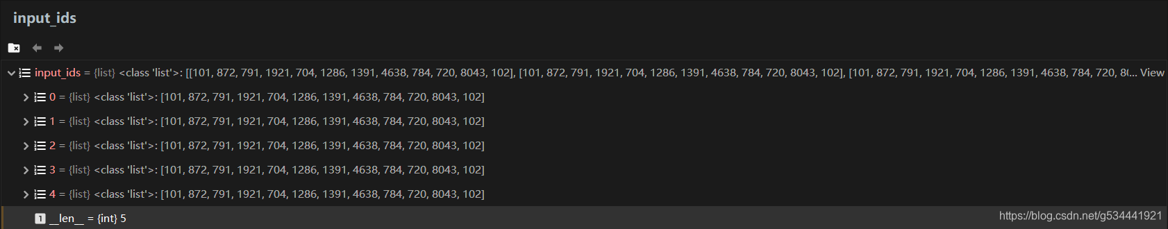
       curr_input_tensors = torch.tensor(input_ids).long().to(device)
       generated = []  # 二维数组,维度为(生成的response的最大长度,batch_size),generated[i,j]表示第j个response的第i个token的id
       finish_set = set()  # 标记是否所有response均已生成结束,若第i个response生成结束,即生成了sep_token_id,则将i放入finish_set
# 最多生成max_len个token
for _ in range(args.max_len):
outputs = dialogue_model(input_ids=curr_input_tensors)
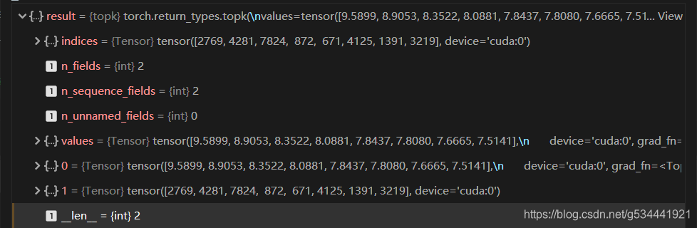
next_token_logits = outputs[0][:, -1, :]
基本没有变化,只提一点,那就是经过正向传播的outputs中5个输出完全相同。
注意:这里是dialogue_model即普通对话模型。
                # 对于已生成的结果generated中的每个token添加一个重复惩罚项,降低其生成概率
                for index in range(args.batch_size):
                    for token_id in set([token_ids[index] for token_ids in generated]):
                        next_token_logits[index][token_id] /= args.repetition_penalty
                next_token_logits = next_token_logits / args.temperature
                # 对于[UNK]的概率设为无穷小,也就是说模型的预测结果不可能是[UNK]这个token
                for next_token_logit in next_token_logits:
                    next_token_logit[tokenizer.convert_tokens_to_ids('[UNK]')] = -float('Inf')
这个部分也是基本相同。
				filtered_logits = top_k_top_p_filtering(next_token_logits, top_k=args.topk, top_p=args.topp)
                # torch.multinomial表示从候选集合中无放回地进行抽取num_samples个元素,权重越高,抽到的几率越高,返回元素的下标
                // 注意,经过multinomial操作,这batch_size个分支就可能抽到不同的字符了。
                next_token = torch.multinomial(F.softmax(filtered_logits, dim=-1), num_samples=1)
如某轮next_token的值为:
tensor([[7649],
        [2769],
        [3219],
        [4281],
        [2769]])
                # 判断是否有response生成了[SEP],将已生成了[SEP]的resposne进行标记
                for index, token_id in enumerate(next_token[:, 0]):
                    if token_id == tokenizer.sep_token_id:
                        finish_set.add(index)
                # 检验是否所有的response均已生成[SEP]
                finish_flag = True  # 是否所有的response均已生成[SEP]的token
                for index in range(args.batch_size):
                    if index not in finish_set:  # response批量生成未完成
                        finish_flag = False
                        break
                if finish_flag:
                    break
简单再做下注解:
set中存放的是已经生成出SEP的回复的序号,比如batch_size为5
我们的起点就是5个完全相同的序列,分别产生输出,每当有一个序列产生了SEP,就将这个序列的index储存进set中,直至所有的index(0~4)都存进了set,本轮生成结束。
                generated.append([token.item() for token in next_token[:, 0]])
                # 将新生成的token与原来的token进行拼接
                curr_input_tensors = torch.cat((curr_input_tensors, next_token), dim=-1)
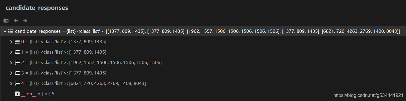
            candidate_responses = []  # 生成的所有候选response
            for batch_index in range(args.batch_size):
                response = []
                for token_index in range(len(generated)):
                    if generated[token_index][batch_index] != tokenizer.sep_token_id:
                        response.append(generated[token_index][batch_index])
                    else:
                        break
                candidate_responses.append(response)
形式如下:
            # mmi模型的输入
            if args.debug:
                print("candidate response:")
            samples_file.write("candidate response:\n")
            min_loss = float('Inf')
            best_response = ""
            for response in candidate_responses:
                mmi_input_id = [tokenizer.cls_token_id]  # 每个input以[CLS]为开头
                mmi_input_id.extend(response)
                mmi_input_id.append(tokenizer.sep_token_id)
                for history_utr in reversed(history[-args.max_history_len:]):
                    mmi_input_id.extend(history_utr)
                    mmi_input_id.append(tokenizer.sep_token_id)
这里和之前一样是将历史对话也读取进来,唯一的区别是将需要读取的历史对话也进行了倒序。
还是为了方便理解:
历史对话:问1 答1 问2 答2 问3
mmi_input 答3(生成的) 问3 答2 问2 答1 问1
                mmi_input_tensor = torch.tensor(mmi_input_id).long().to(device)
                out = mmi_model(input_ids=mmi_input_tensor, labels=mmi_input_tensor)
转成tensor后送入mmi_model中进行前向计算(这次是mmi_model!)
来看下out的形式:
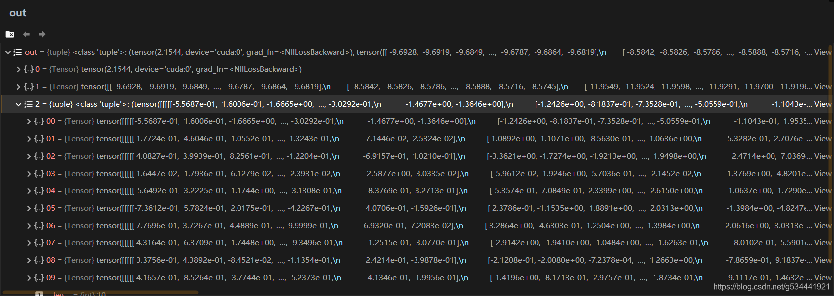
[0]: loss值
[1]: shape:torch.Size([46, 13317])
[2,0]: shape:torch.Size([2, 1, 12, 46, 64])
为什么是46呢,因为mmi_input_tensor的shape刚好是46。
                loss = out[0].item()
                if args.debug:
                    text = tokenizer.convert_ids_to_tokens(response)
                    print("{} loss:{}".format("".join(text), loss))
                samples_file.write("{} loss:{}\n".format("".join(text), loss))
                if loss < min_loss:
                    best_response = response
                    min_loss = loss
取loss最小的作为最佳回复。
            history.append(best_response)
            text = tokenizer.convert_ids_to_tokens(best_response)
            print("chatbot:" + "".join(text))
            if args.save_samples_path:
                samples_file.write("chatbot:{}\n".format("".join(text)))
        except KeyboardInterrupt:
            if args.save_samples_path:
                samples_file.close()
            break
到这里对本项目的详细流程调试就基本结束了,最后说一点我本人的疑问:
项目作者总是将输入作为label,我总觉得这样做虽然也可以产生不差的效果,但与原论文中所阐述的,用答句来预测问句还是有一定区别的。我谨以为相应的部分需要稍微改进一下,将前向计算的label设为输入对话之前的问答部分,不过重在学习项目本身,感兴趣的朋友可以自行尝试。如果是我理解有误还请评论指出!
