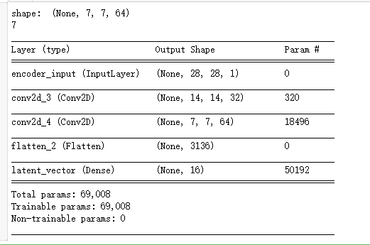
from keras.layers import Dense, Input
from keras.layers import Conv2D, Flatten
from keras.layers import Reshape, Conv2DTranspose
from keras.models import Model
from keras.datasets import mnist
from keras import backend as K

import numpy as np
import matplotlib.pyplot as plt

#加载手写数字图片数据
(x_train, _), (x_test, _) = mnist.load_data()
image_size = x_train.shape[1]


#把图片大小统一转换成28*28,并把像素点值都转换为[0,1]之间
x_train = np.reshape(x_train, [-1, image_size, image_size, 1])
x_test = np.reshape(x_test, [-1, image_size, image_size, 1])
x_train = x_train.astype('float32') / 255
x_test = x_test.astype('float32') / 255

input_shape = (image_size, image_size, 1)
batch_size = 32
#对图片做3*3分割
kernel_size = 3
#让编码器将输入图片编码成含有16个元素的向量
latent_dim = 16
inputs = Input(shape=input_shape, name='encoder_input')
x = inputs
'''
编码器含有两个卷积层,第一个卷积层将每个3*3切片计算成含有32个元素的向量,第二个卷积层将3*3切片
计算成含有64个元素的向量
'''

layer_filters = [32, 64]
for filters in layer_filters:
  #stride=2表明每次挪到2个像素,如此一来做一次卷积运算后输出大小会减半
  x = Conv2D(filters = filters, kernel_size = kernel_size, activation='relu',
            strides = 2,
            padding = 'same')(x)

shape = K.int_shape(x)
print('shape: ', shape)
print(shape[1])
x = Flatten()(x)
#最后一层全连接网络输出含有16个元素的向量
latent = Dense(latent_dim, name = 'latent_vector')(x)
encoder = Model(inputs, latent, name='encoder')
encoder.summary()
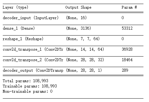
#构造解码器,解码器的输入正好是编码器的输出结果
latent_inputs = Input(shape = (latent_dim, ), name = 'decoder_input')
'''
它的结构正好和编码器相反,它先是一个全连接层,然后是两层反卷积网络
'''
x = Dense(shape[1] * shape[2] * shape[3])(latent_inputs)
x = Reshape((shape[1], shape[2], shape[3]))(x)


#两层与编码器对应的反卷积网络
for filters in layer_filters[::-1]:
  x = Conv2DTranspose(filters = filters, kernel_size = kernel_size,
                    activation='relu', strides = 2,
                    padding = 'same')(x)


outputs = Conv2DTranspose(filters = 1, kernel_size = kernel_size,
                          activation = 'sigmoid',
                          padding = 'same',
                          name = 'decoder_output')(x)
decoder = Model(latent_inputs, outputs, name = 'decoder')
decoder.summary()
autoencoder = Model(inputs, decoder(encoder(inputs)), name = 'autoencoder')
autoencoder.summary()

'''
网络训练时,我们采用最小和方差,也就是我们希望解码器输出的图片与输入编码器的图片,在像素上的差异
尽可能的小
'''
autoencoder.compile(loss='mse', optimizer='adam')
autoencoder.fit(x_train, x_train, validation_data=(x_test, x_test),
               epochs = 1,
               batch_size = batch_size)

'''
x_test是输入编码器的测试图片,我们看看解码器输出的图片与输入时是否差别不大
'''
x_decoded = autoencoder.predict(x_test)
#把测试图片集中的前8张显示出来,看看解码器生成的图片是否与原图片足够相似
imgs = np.concatenate([x_test[:8], x_decoded[: 8]])
imgs = imgs.reshape((4, 4, image_size, image_size))
imgs = np.vstack([np.hstack(i) for i in imgs])
plt.figure()
plt.axis('off')
plt.title('Input: 1st 2 rows, Decoded: last 2 rows')
plt.imshow(imgs, interpolation='none', cmap='gray')
plt.show()

