在看完第一篇的情况下,这一篇给人的感觉就算灌水严重。。。主要内容集中在相似度测量方面的过程和为了加速运算在内存管理方面的额外并行化处理,depth方面的内容和第一篇相同就没有摘录了
这是基于linemod的第三篇文章,主要集中于他们提出的相似度检测这一点的阐述方面
- Similarity Measure:
unoptimized similarity measure is : \(\varepsilon_{Steger}(I,T,c)=\sum_{r\in P}\left| cos(ori(O,r)- ori(I,c+r))\right|\), where \(ori(O,r)\) is the gradient orientation in radians at location \(r\) in a reference image \(O\) of an object to detect. \(ori(I, c+r)\) is the gradient orientation at \(c\) shifted by \(r\) in the input image \(I\). Use a list \(P\) to define the location \(r\) to be considered in \(O\). So template \(T = (O, P)\). the Eq. is robust to background clutter, but not to small shifts and deformations. So we introduce a similarity measure that, for each gradient orientation on the object, searches in a neighborhood of the associated gradient location for the most similar orientation in the input image. And Eq is formalized as: \(\varepsilon(I,T,c)=\sum_{r\in P}(\max_{t\in R(c+r)}\left| cos(ori(O,r)- ori(I,c+r))\right|)\) where \(R(c+r) = [c+r-\frac{T}{2}, c+r+\frac{T}{2}]\times[c+r-\frac{T}{2}, c+r+\frac{T}{2}]\). To increase robustness, for each image location use the gradient orientation of the channel whose magnitude is largest. Given an RGB color image \(I\), we compute the gradient orientation map \(I_G(x)\) at location \(x\) with \(I_G(x) = ori(\hat{C}(x))\) where \(\hat{C}(x) = \arg\max_{C\in \{R,G,B\}}\left\| \frac{\vartheta C}{\vartheta x} \right\|\) - Spreading the Orientations:
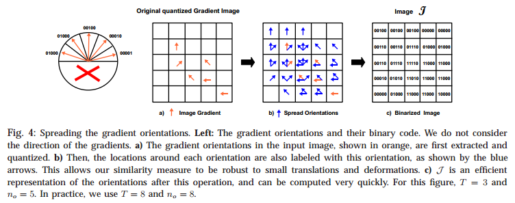
a binary representation \(J\) of the gradient around each image location. First, we quantize orientations into a small number of \(n_0\) values. And spread the gradient of input image around their locations to obtain a new representation of the original image. Each individual bit of this string corresponds to one quantized orientation, and is set to 1 if this orientation is present in the \([-\frac{T}{2}, \frac{T}{2}] \times [-\frac{T}{2}, \frac{T}{2}]\)neighborhood of \(m\). The string will be used as indices to access lookup tables. - Precomputing Response Maps:

\(J\) is used together with lookup tables to precompute the value of the max operation for each location and each possible orientation \(ori(O, r)\) in the tamplate. We store the results into 2D maps \(S_i\). And we use \(\tau_i\) for each of the \(n_0\) quantized orientations and compute as: \(\tau_i[L]=\max_{l\in L}\left| cos(i-l)\right|\), where \(i\) is the index of quantized orientations, \(L\) is the list of orientations appearing in local neighborhood of a gradient with oridientation \(i\). For each orientttion \(i\), we can now compute the value at each location \(c\) of the response map \(S_i\) as: \(S_i(c)=\tau_i[J(c)]\). And now we can get \(\varepsilon(I, T, c)=\sum_{r\in P}S_{ori(O,r)}(c+r)\) - Linearizing the Memory for Parallelization:
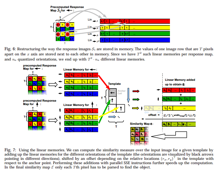
We restructure each response map so that the values of one row that are \(T\) pixels apart on the \(x\) axis are now stored next to each other in memory. We continue with the row which is \(T\) pixels apart on the \(y\) axis once we finished with the current one.