Portfolio analysis
Abstract
The construction of investment portfolio is a perennial question in the analysis of financial investment. For years, the academic field and the industrial field have proposed many ways to optimize the portfolio. The theory of Markowitz mean-variance model (M-V model) takes the primary place. In the first part, this report introduces a method of constructing an effective stock portfolio with M-V model to establish effective frontier by using R. In the second part, we have built a simple simulation trading system for one stock by using R.
Content
1 Construct portfolio 1
1.1 Introduction 1
1.2 portfolio construction 2
1.3 evaluation 3
2 trading system 4
2.1 methodology 4
2.2 a trading system with one MA line 4
2.3 a trading system with two MA lines 6
3 conclusion 7
1 Construct portfolio
1.1 Introduction
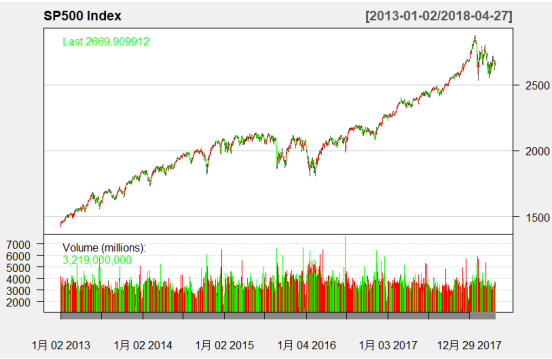
The Standard & Poor’s 500 (abbreviated as S&P500), is an American stock market index based on the market capitalizations of 500 large companies having common stock listed on NYSE or NASDAQ. The S&P500 index has experienced a circle of bull market and bear market since 2013. So our sample encompasses a over 5-year period from January 2013 to April 2018.
1.2 portfolio construction
Companies like GOOGLE, IBM, MICROSOFT, APPLE and FACEBOOK are labeled as IT constitutes of S&P500 components. Companies like AFFIL MANAGERS, GOLDMAN SACHS, Citi Group, NASDAQ and MOODYS are labeled as financial constitutes of S&P500 components.
By R command getSymbols(), we get the historical market data of the ten stocks mentioned above and S&P500 index from yahoo finance website.
Supposing that one company can continue operating for more than 10 years, so we take 10-year US treasury interest rate as risk-free rate.
For simple, we construct two equal weighted portfolios:

The correlation matrix of IT stocks and S&P500 is listed as below.
GOOG/ MSFT/AAPL/FB are highly correlated with each other, IBM is negative correlated with other 4 stocks.
| GOOG |
IBM |
MSFT |
AAPL |
FB |
SPY |
|
| GOOG |
1.00 |
-0.23 |
0.98 |
0.89 |
0.97 |
0.95 |
| IBM |
-0.23 |
1.00 |
-0.19 |
-0.29 |
-0.31 |
-0.21 |
| MSFT |
0.98 |
-0.19 |
1.00 |
0.92 |
0.96 |
0.97 |
| AAPL |
0.89 |
-0.29 |
0.92 |
1.00 |
0.93 |
0.97 |
| FB |
0.97 |
-0.31 |
0.96 |
0.93 |
1.00 |
0.97 |
| SPY |
0.95 |
-0.21 |
0.97 |
0.97 |
0.97 |
1.00 |
1.3 evaluation
The capital asset pricing model(CAPM), derived by Sharpe, Lintner and Mossin, is one of the most celebrated models in all of finance. The model describes the relationship we should expect to see between risk and return for individual assets. Specifically, the CAPM provides a way to calculate an asset’s expected return (or “required” return) based on its level of systematic (or market-related) risk, as measured by the asset’s beta.
For a portfolio, the equation for CAPM is

Which ![]() is the risky free rate,
is the risky free rate, ![]() stands for the return of market,
stands for the return of market, ![]() represents the sensitivity of the portfolio’s return to the market return.
represents the sensitivity of the portfolio’s return to the market return.
Through linear regression, R command without intercept  , we can get the beta of two portfolios:

Beta is considered as the systematic risk, in a diversified portfolio, an investor should only be compensated for systematic risk (or beta) exposure. Beta reflects the relationship between the portfolio and the whole market. If beta is larger than 1, the portfolio earns more when the market goes up. If beta is smaller than 1, the portfolio loses less when the market goes down.
Form the linear regression results, we can see portfolio 1 and portfolio 2 both have beta greater than 1. When the market goes up, the portfolios will earn more than the market.
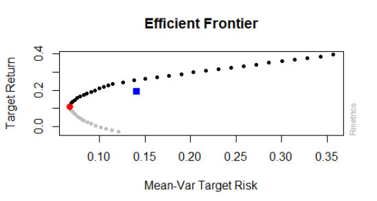
Future, we want to calculate the efficient frontier. take portfolio 1 as example.
the efficient frontier is shown as below, the red point represents the minimum risk portfolio, the blue point represents the equal weights portfolio. it’s obvious that equal weights portfolio is not on the efficient frontier.
2 trading system
2.1 methodology
Moving average(MA) line is the most common technical analysis method in stock market. People use MA to look for trading signals in stock market. MA is simple and effective. In technical analysis field, moving average line is a necessary index tool. There are 3 main moving average line in application.
1) Simple moving average (SMA)
2) Weighted moving average(WMA)
3) Exponential moving average(EMA)
MA line are always smoothness, we can see there are some crosses between MA line and candlestick charts. those crosses will help us to judge trading signals whether to buy or to sell. In this report, we want to trade GOOGLE for example.
2.2 a trading system with one MA line
The main design thought:
1) if the close price of the stock up-cross the 20-day MA line, buy it
2) if the close price of the stock down-cross the 20-day MA line, sell it
At first, we write our own moving average function ma(), and the custom function about drawing moving average lines drawLine().
The MA20 lines are defined on the barchart of GOOGLE.
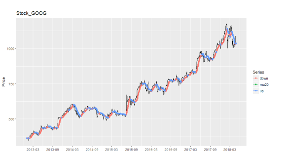
drawPoint() function will mark the holding times and empty times with different color. Then we can see that when close price is less than MA20, will be shown in red, when close price is greater than MA20, will be shown in blue. Then we can buy in the stock when the first red point occurs, and sell out the stock when the first blue point occurs. This process will come to a simple trading system.
Then we try to find out those trading points and calculate whether the tradings actually earn money or loss money. The function signal() and trade()are designed to find out this question. we find that there are 154 times trading logs, half is the buy actions.
Set initial capital equals 1 million, suppose that we fully invested at all times, and with no trade cost. Through simulation trading, we can actually calculate the performance the strategy.
> tail(result1$ticks,1)
Value op cash amount asset diff
2018-04-26 1040.04 B 715.5761 168 175442.3 0
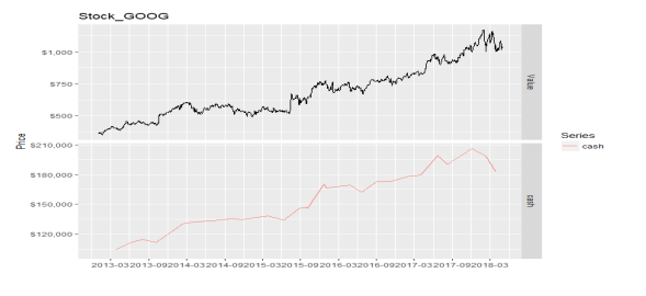
Through the above output, we can know that on 2018-04-26, the strategy suggests to buy in, and the total profit is 75442.3. the number of profit operations is 24, the number of loss operation is 52. Why we still earn money in the end? We draw the cash flow over the whole trading period shown below.
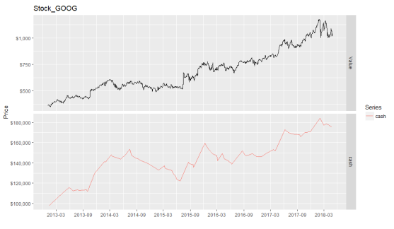
In the long going-up trends, the trading operations have earned a lot of money. But when the market is fluctuated, the strategy will loss efficacy and have a big drawdown, which can be seen during 2014-03 ~ 2015-06. The maxdrawdown is 31%.
2.3 a trading system with two MA lines
One moving average line will earn money during long going-up trends. but we must realize that one MA line system is very sensitive to fluctuations. If small fluctuations are too frequent, not only will the number of transactions be increased, but the model will fail.
We introduce this method, some like one MA line.
1) Get MA12, MA26
2) If MA12 up-cross MA26, buy (gold cross)
3) If MA12 down-cross MA26, sell (dead cross)
Still take GOOGLE as the test sample. We count that there are 18 times trading ended with profit, and 10 times trading ended with loss. two-line will reduce the number of signal.
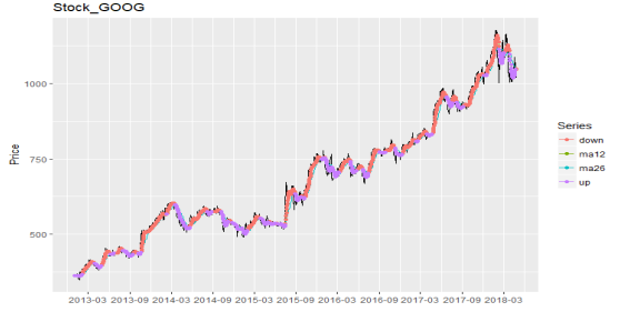
> tail(result2$ticks,1)
Value op cash amount asset diff
2018-04-24 1019.98 B 277.5063 179 182853.9 0
The final P&L is 82853.9. two-line system produces less trading signal than one-line system. The maxdrawdown is 23%, which is smaller than the one-line system. Two-line system is more stable than one-line system.
3 conclusion
In this report, we compare different portfolios with CAPM, the IT portfolio and finance portfolio are both outperform S&P500 index. We build a simple trading system with moving average lines. To simplify the processing, we assume no transaction costs, and this system only trade one stock. If we want to trade a set of stock, we should do more work to develop the program.
这是我写的关于期末报告!
Report on Portfolio Analysis
Introduction
Portfolio analysis has always been an interesting and absorbing topic in the study of Finance. One of the fundamental question in Finance is how to tradeoff between profit and risk. Markowitz (1952) provides the first systematic method for solving the problem, which revolutionize the study of Finance. In his paper, he proposes a mean-variance approach to set up a model that are both general enough for practical situations and simple enough to be numerically solved, which serves as a classic framework for the study of portfolio analysis. Another fundamental question in Finance is to price assets under uncertainty. The Capital Asset Pricing Model (CAPM) proposed by Sharpe (1964) and Lintner (1965) provides a start point and a benchmark in answering this question. About fifty years later, Capital Asset Pricing Model (CAPM) is still widely used both theoretically and practically. When evaluating the performance of portfolios, Capital Asset Pricing Model (CAPM) still provides one of the most useful framework.
In this report, I will conduct a portfolio analysis from two parts. In the first part, I will construct stock portfolios and compare their performance within the framework of Capital Asset Pricing Model (CAPM). In the second part, I will propose a trading strategy and evaluate its performance on the market.
The Construction of Portfolios
In this section, I will construct two portfolios of stocks and compare their performance.
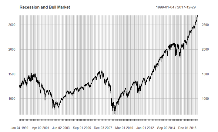
The data I use is from January 2001 to January 2018, which cover the periods of recession and bull market. Here I use the return of S&P500 as an indicator for recession and bull market. When the yearly return of S&P500 is greater than 20%, I define the year as bull market year. When the yearly return of S&P500 is less than -20%, I define the year as recession year. Based on this criterion, year 2002 and year 2008 are the recession year. In year 2002, the bubble of Internet company bursts, which leads to a great decrease in stock market. In year 2008, the great recession begins, which causes a huge plunge in stock market. In year 2003, year 2009, year 2013, the stock market begins to recover and the yearly returns of S&P500 are greater than 20%, suggests a bull market starts to form. The returns of S&P 500 are depicted in the following figure.
To construct the portfolio, I choose the firms which have a relatively long history of data. That is, I will focus on the firms who have the data at least cover the period of January 2001 to January 2018. In this report, I will construct two main portfolios. The first portfolio is comprised of the most prestigious firms of various traditional industries. To be specific, I choose the stocks of five traditional companies that comes from different industries in the first portfolio, they are Coca-Cola Company, AT&T company, Walmart company, Ford company and CVS company. The second portfolio is comprised of the most prestigious firms of high technology. To be specific, I choose the stocks of five high technology companies in the second portfolio, they are Apple company, IBM company, Microsoft company, Intel company and CISCO company. A simple and natural way to construct the portfolios is to set weights to be the equal for all the companies in the two portfolios. The yearly return of the two portfolios are as follows
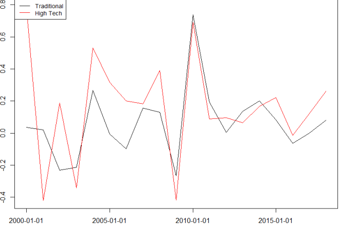
We can see the high technology portfolio generally has a higher return and higher volatility
than traditional portfolio.
Evaluation under CAPM
After constructing the portfolios, we can evaluate their performance under the framework
of Capital Asset Pricing Model (CAPM).
The Capital Asset Pricing Model (CAPM) can be expressed as follows


is the market return rate, in this report, I use S&P 500 to proxy for the market return rate, ![]() is the risk free rate, I use the rate of 3-Month Treasury Bill to proxy for the risk free rate.
is the risk free rate, I use the rate of 3-Month Treasury Bill to proxy for the risk free rate.
After calculating in R, we get the beta for the traditional portfolio is 0.9689, the beta for the high technology portfolio is 1.4215. These results suggest that the traditional portfolio we choose is quite close to the S&P 500 and the high technology portfolio is more aggressive than the traditional portfolio.
A good measure for the performance of portfolios is Sharpe Ratio, which measures the average excess return to the risk per unit. Sharpe Ratio is expressed as

After calculating in R, we get the Sharpe Ratio for the traditional portfolio is 0.1348, the Sharpe Ratio for the high technology portfolio is 0.4090. These results suggest that the high technology portfolio has a much higher risk-adjusted excess return than that of traditional portfolio.
Another index which is useful for evaluating the performance of portfolios is Jensen’s alpha, which is used to measure the abnormal return of a portfolio over the theoretical expected return. Jensen’s alpha is expressed as follows.

After calculating in R, we get the Jensen’s alpha for the traditional portfolio is 0.0046, the Jensen’s alpha for the high technology portfolio is 0.0953. These suggest that the high technology portfolio has a much higher abnormal return than traditional portfolio.
Therefore, based on the CAPM framework, the high technology portfolio has a better performance than traditional portfolio. Note that we may assign weights based on previous information for the portfolios to improve their performance. This is can be further studied in the future.
Trading Strategy
In this section, I will propose a trading strategy and evaluate its performance on the stock market. Technical analysis method is used on constructing the trading strategies.
Here I will use the stock of Apple company as an example for the trading strategies. The strategies we use are mainly based on the indicator of Moving Average Convergence Divergence (MACD) and Bollinger bands (BB). I will propose two trading strategy based on these two indicators. I choose closing price of the stock of Apple to calculate the averages. The trading strategy is simulated on the data between January 2016 to December 2017. Note that technical trading strategies only use past trading information on the analysis and the information is known when we make transactions based on the t technical trading strategies. It is not so necessary to leave some data out of sample. So, we do the simulation with the data of most recent two years.
In the trading strategy based on Moving Average Convergence Divergence (MACD), two averages of closed prices are computed at first: a slow-moving average and a fast-moving average. The difference between the them is called MACD line. We also need to calculate the third average: a 9-day exponential moving average of MACD, this third average is used as MACD signal line. If the MACD line crosses above the signal line then it is a buying sign and we buy the stock. If the MACD line crosses below the signal line then it is a selling sign and we sell the stock.
To be specific, my Moving Average Convergence Divergence (MACD) trading strategy is to buy 1 share of Apple stock if yesterday’s closed is higher than the signal line and sell it at the end of the day, and to sell 1 share of Apple stock if yesterday’s closed is lower than the signal line and close the short position at the end of the day. Assuming no transaction cost, the result of the trading strategy is as follows
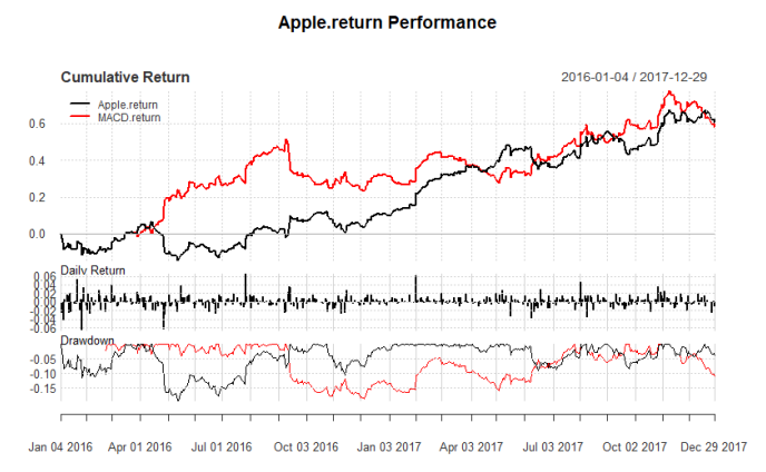
From the result, we can see that our trading strategy provides a cumulative return tends to be even better than the cumulative return of Apple stock. Note that Apple stock gives a return of about 10% in 2016, but with my trading strategy, the return is about 30%. In most of the time, the return of this trading strategy provides a return even higher than Apple stock. With this trading strategy, the cumulative return is about 60% for just two years, which is quite high.
Bollinger bands (BB) analyzes the band around the price movements of an asset. The band is based on standard deviations and a moving average. Bollinger bands have three lines, upper, middle and lower. The middle line is a moving average of prices. Bollinger bands help analyze how strongly the price is rising, and when the stock is potentially losing strength or reversing the trend. My Bollinger bands (BB) trading strategy is to buy 1 share of Apple stock if yesterday’s closed is higher than the middle line and sell it at the end of the day, and to sell 1 share of Apple stock if yesterday’s closed is lower than the middle line and close the short position at the end of the day. Assuming no transaction cost, the result of the trading strategy is as follows
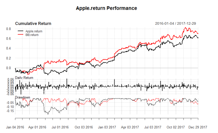
We can see that the Bollinger bands (BB) trading strategy provides a return which is almost consistently higher than the return of Apple stock. With this trading strategy, the cumulative return is about 70% for just two years, which is even higher than the Moving Average Convergence Divergence (MACD) trading strategy. The volatility of the returns from Bollinger bands (BB) trading strategy tends also to be lower than that of Moving Average Convergence Divergence (MACD) trading strategy.
Conclusion
In this report, I first use the framework of Capital Asset Pricing Model (CAPM) to evaluate the performance of two portfolio: one is comprised of traditional firms, the other is comprised of high technology firms. The result shows that high technology portfolio tends to have better performance than traditional portfolio under the framework of Capital Asset Pricing Model (CAPM) in the sense that it has a higher Sharpe Ratio and higher Jensen’s Alpha.
Then I propose two trading strategies based on Moving Average Convergence Divergence (MACD) and Bollinger bands (BB). The simulation results show that the two trading strategies tend to have better performance than the return of Apple stock. But, we may need to note that the performance of short term trading strategy may depend on the stock it chooses and the condition of market. For more general trading strategies, further researches may be needed.
Reference
Lintner, J. (1965). Security prices, risk, and maximal gains from diversification. The journal of finance, 20(4), 587-615.
Markowitz, H. (1952). Portfolio selection. The journal of finance, 7(1), 77-91.
Sharpe, W. F. (1964). Capital asset prices: A theory of market equilibrium under conditions of risk. The journal of finance, 19(3), 425-442.
天才写手,代写CS,代写finance,代写statistics,北美代写
出自:https://uhomework.com/a/R/20180628/16437.html