数据挖掘题目：设ε= 2倍的格网间距，MinPts = 6, 采用基于1-范数距离的DBSCAN算法对下图中的实心格网点进行聚类，并给出聚类结果（代码解答）

问题

代码

import matplotlib.pyplot as plt
import numpy as np
from sklearn.cluster import DBSCAN
#pip install matplotlib
#pip install numpy
#pip install scikit-learn
# 实心格网点的坐标
solid_points = np.array([[1, 1], [2, 1],[3, 1], [1, 2], [2, 2], [3, 2],[1, 3],[3, 3], [1, 4],[3, 4], [1, 5], [2, 5], [3, 9], [6, 4],[7, 6], [7, 7], [7, 8], [7, 9], [8, 6], [9, 7], [9, 8], [9, 9] ,[10, 6],[11, 6],[11, 7],[11, 8],[11, 9]])


# 执行DBSCAN聚类
'''
对于1范数（曼哈顿距离），将metric参数的值设置为'manhattan'：
dbscan = DBSCAN(eps=2, min_samples=6, metric='manhattan')
对于2范数（欧几里德距离），将metric参数的值设置为'euclidean'：
dbscan = DBSCAN(eps=2, min_samples=6, metric='euclidean')
对于无穷范数，将metric参数的值设置为'chebyshev'：
dbscan = DBSCAN(eps=2, min_samples=6, metric='chebyshev')
'''
dbscan = DBSCAN(eps=2, min_samples=6, metric='manhattan')
labels = dbscan.fit_predict(solid_points)


# 获取核心点的索引
core_samples_mask = np.zeros_like(labels, dtype=bool)
core_samples_mask[dbscan.core_sample_indices_] = True
core_indices = np.where(core_samples_mask)[0]

# 获取边缘点的索引
border_indices = np.setdiff1d(np.where(labels != -1)[0], core_indices)

# 获取孤立点的索引
outlier_indices = np.where(labels == -1)[0]


# 映射字典
mapping  = {
    
    
    1: 'A',
    2: 'B',
    3: 'C',
    4: 'D',
    5: 'E',
    6: 'F',
    7: 'G',
    8: 'H',
    9: 'I',
    10: 'J',
    11: 'K'
}

# 构建簇与点的映射关系
clusters = {
    
    }
for i, label in enumerate(labels):
    clusters.setdefault(label, {
    
    'core': [], 'border': []})
    if label != -1:
        if i in core_indices:
            clusters[label]['core'].append(solid_points[i])
        else:
            clusters[label]['border'].append(solid_points[i])

# 打印各个簇的核心点和边界点
for label, cluster in clusters.items():
    core_points = [f"{
      
      mapping[point[0]]}{
      
      point[1]}" for point in cluster['core']]
    border_points = [f"{
      
      mapping[point[0]]}{
      
      point[1]}" for point in cluster['border']]
    if label!=-1:
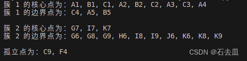
        print(f"簇 {
      
      label+1} 的核心点为：" + ", ".join(core_points))
        print(f"簇 {
      
      label+1} 的边界点为：" + ", ".join(border_points))
        print()

# 打印孤立点
outliers = [f"{
      
      mapping[point[0]]}{
      
      point[1]}" for point in solid_points[outlier_indices]]
print("孤立点为：" + ", ".join(outliers))
print()

# 绘制实心格网点和空心格网点的聚类结果
# 先获取当前的坐标轴
ax = plt.gca()
# 将y轴方向进行翻转
ax.invert_yaxis()
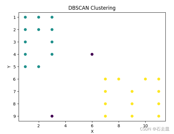
# 绘制散点图
plt.scatter(solid_points[:, 0], solid_points[:, 1], c=labels)
plt.xlabel('X')
plt.ylabel('Y')
plt.title('DBSCAN Clustering')
plt.show()

结果