点击进入专栏:
《人工智能专栏》 Python与Python | 机器学习 | 深度学习 | 目标检测 | YOLOv5及其改进 | YOLOv8及其改进 | 关键知识点 | 各种工具教程
文章目录
解读预训练与微调迁移,模型冻结与解冻
官方文档:
https://docs.ultralytics.com/yolov5/tutorials/transfer_learning_with_frozen_layers/#freeze-backbone
一个完整的代码
pythonCopy codeimport torch
import torchvision
import torchvision.transforms as transforms
import torch.nn as nn
import torch.optim as optim
# 设置设备(CPU或GPU)
device = torch.device("cuda" if torch.cuda.is_available() else "cpu")
# 定义预训练模型
pretrained_model = torchvision.models.resnet18(pretrained=True)
pretrained_model.to(device)
# 冻结预训练模型的参数
for param in pretrained_model.parameters():
    param.requires_grad = False
# 替换最后一层全连接层
num_classes = 10 # 分类任务的类别数
pretrained_model.fc = nn.Linear(pretrained_model.fc.in_features, num_classes)
pretrained_model.fc.to(device)
# 加载训练数据集
transform = transforms.Compose([
    transforms.Resize((224, 224)),
    transforms.ToTensor(),
    transforms.Normalize((0.5, 0.5, 0.5), (0.5, 0.5, 0.5))
])
train_dataset = torchvision.datasets.CIFAR10(root='./data', train=True, download=True, transform=transform)
train_loader = torch.utils.data.DataLoader(train_dataset, batch_size=32, shuffle=True)
# 定义损失函数和优化器
criterion = nn.CrossEntropyLoss()
optimizer = optim.SGD(pretrained_model.parameters(), lr=0.001, momentum=0.9)
# 训练模型
num_epochs = 10
for epoch in range(num_epochs):
    total_loss = 0.0
    correct = 0
    total = 0
    for images, labels in train_loader:
        images = images.to(device)
        labels = labels.to(device)
        optimizer.zero_grad()
        # 前向传播
        outputs = pretrained_model(images)
        loss = criterion(outputs, labels)

        # 反向传播和优化
        loss.backward()
        optimizer.step()
        total_loss += loss.item()
        _, predicted = outputs.max(1)
        total += labels.size(0)
        correct += predicted.eq(labels).sum().item()
    # 打印训练信息
    print('Epoch [{}/{}], Loss: {:.4f}, Accuracy: {:.2f}%'
          .format(epoch+1, num_epochs, total_loss/len(train_loader), 100*correct/total))
预训练与微调迁移
1. 什么是预训练和微调
- 你需要搭建一个网络模型来完成一个特定的图像分类的任务。首先,你需要随机初始化参数,然后开始训练网络,不断调整参数,直到网络的损失越来越小。在训练的过程中,一开始初始化的参数会不断变化。当你觉得结果很满意的时候,你就可以将训练模型的参数保存下来,以便训练好的模型可以在下次执行类似任务时获得较好的结果。这个过程就是
pre-training。 - 之后,你又接收到一个类似的图像分类的任务。这时候,你可以直接使用之前保存下来的模型的参数来作为这一任务的初始化参数,然后在训练的过程中,依据结果不断进行一些修改。这时候,你使用的就是一个
pre-trained模型,而过程就是fine-tuning。
所以,预训练 就是指预先训练的一个模型或者指预先训练模型的过程;微调 就是指将预训练过的模型作用于自己的数据集,并使参数适应自己数据集的过程。
1.1 预训练模型
- 预训练模型就是已经用数据集训练好了的模型。
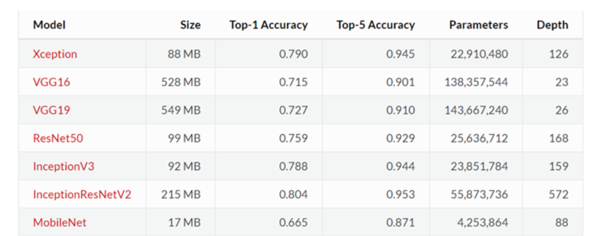
- 现在我们常用的预训练模型就是他人用常用模型,比如
VGG16/19,Resnet等模型,并用大型数据集来做训练集,比如Imagenet, COCO等训练好的模型参数; - 正常情况下,我们常用的
VGG16/19等网络已经是他人调试好的优秀网络,我们无需再修改其网络结构。
2. 预训练和微调的作用
在 CNN 领域中,实际上,很少人自己从头训练一个 CNN 网络。主要原因是自己很小的概率会拥有足够大的数据集,基本是几百或者几千张,不像 ImageNet 有 120 万张图片这样的规模。拥有的数据集不够大,而又想使用很好的模型的话,很容易会造成过拟合。
所以,一般的操作都是在一个大型的数据集上(ImageNet)训练一个模型,然后使用该模型作为类似任务的初始化或者特征提取器。比如 VGG,ResNet 等模型都提供了自己的训练参数,以便人们可以拿来微调。这样既节省了时间和计算资源,又能很快的达到较好的效果。
3. 模型微调
3.1 微调的四个步骤
- 在源数据集(例如 ImageNet 数据集)上预训练一个神经网络模型,即源模型。
- 创建一个新的神经网络模型,即目标模型。它复制了源模型上除了输出层外的所有模型设计及其参数。我们假设这些模型参数包含了源数据集上学习到的知识,且这些知识同样适用于目标数据集。我们还假设源模型的输出层跟源数据集的标签紧密相关,因此在目标模型中不予采用。
- 为目标模型添加一个输出大小为目标数据集类别个数的输出层,并随机初始化该层的模型参数。
- 在目标数据集(例如椅子数据集)上训练目标模型。我们将从头训练输出层,而其余层的参数都是基于源模型的参数微调得到的。

3.2 为什么要微调
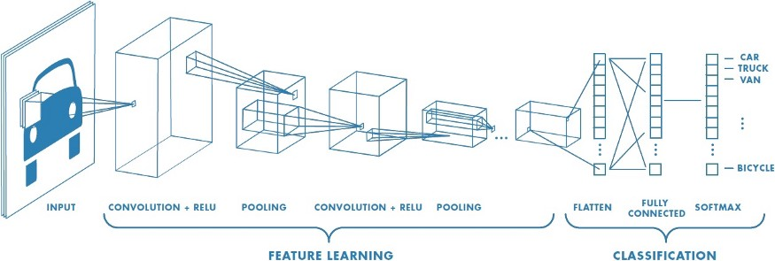
卷积神经网络的核心是:
- 浅层卷积层提取基础特征,比如边缘,轮廓等基础特征。
- 深层卷积层提取抽象特征,比如整个脸型。
- 全连接层根据特征组合进行评分分类。
普通预训练模型的特点是:用了大型数据集做训练,已经具备了提取浅层基础特征和深层抽象特征的能力。
如果不做微调的话:
- 从头开始训练,需要大量的数据,计算时间和计算资源。
- 存在模型不收敛,参数不够优化,准确率低,模型泛化能力低,容易过拟合等风险。
3.3 什么情况下使用微调
- 要使用的数据集和预训练模型的数据集相似。如果不太相似,比如你用的预训练的参数是自然景物的图片,你却要做人脸的识别,效果可能就没有那么好了,因为人脸的特征和自然景物的特征提取是不同的,所以相应的参数训练后也是不同的。
- 自己搭建或者使用的CNN模型正确率太低。
- 数据集相似,但数据集数量太少。
- 计算资源太少。
不同数据集下使用微调
- 数据集1 - 数据量少,但数据相似度非常高 - 在这种情况下,我们所做的只是修改最后几层或最终的
softmax图层的输出类别。 - 数据集2 - 数据量少,数据相似度低 - 在这种情况下,我们可以冻结预训练模型的初始层(比如k层),并再次训练剩余的(n-k)层。由于新数据集的相似度较低,因此根据新数据集对较高层进行重新训练具有重要意义。
- 数据集3 - 数据量大,数据相似度低 - 在这种情况下,由于我们有一个大的数据集,我们的神经网络训练将会很有效。但是,由于我们的数据与用于训练我们的预训练模型的数据相比有很大不同。使用预训练模型进行的预测不会有效。因此,最好根据你的数据从头开始训练神经网络(Training from scatch)。
- 数据集4 - 数据量大,数据相似度高 - 这是理想情况。在这种情况下,预训练模型应该是最有效的。使用模型的最好方法是保留模型的体系结构和模型的初始权重。然后,我们可以使用在预先训练的模型中的权重来重新训练该模型。
3.4 微调注意事项
- 通常的做法是截断预先训练好的网络的最后一层(softmax层),并用与我们自己的问题相关的新的softmax层替换它。例如,ImageNet上预先训练好的网络带有1000个类别的softmax图层。如果我们的任务是对10个类别的分类,则网络的新softmax层将由10个类别组成,而不是1000个类别。然后,我们在网络上运行预先训练的权重。确保执行交叉验证,以便网络能够很好地推广。
- 使用较小的学习率来训练网络。由于我们预计预先训练的权重相对于随机初始化的权重已经相当不错,我们不想过快地扭曲它们太多。通常的做法是使初始学习率比用于从头开始训练(Training from scratch)的初始学习率小10倍。
- 如果数据集数量过少,我们进来只训练最后一层,如果数据集数量中等,冻结预训练网络的前几层的权重也是一种常见做法。这是因为前几个图层捕捉了与我们的新问题相关的通用特征,如曲线和边。我们希望保持这些权重不变。相反,我们会让网络专注于学习后续深层中特定于数据集的特征。
4. 迁移学习
迁移学习(Transfer Learning)是机器学习中的一个名词,也可以应用到深度学习领域,是指一种学习对另一种学习的影响,或习得的经验对完成其它活动的影响。迁移广泛存在于各种知识、技能与社会规范的学习中。
通常情况下,迁移学习发生在两个任务之间,这两个任务可以是相似的,也可以是略有不同。在迁移学习中,源任务(Source Task)是已经训练好的模型的来源,目标任务(Target Task)是我们希望在其中应用迁移学习的新任务。
迁移学习专注于存储已有问题的解决模型,并将其利用在其他不同但相关问题上。比如说,用来辨识汽车的知识(或者是模型)也可以被用来提升识别卡车的能力。计算机领域的迁移学习和心理学常常提到的学习迁移在概念上有一定关系,但是两个领域在学术上的关系非常有限。
4.1 迁移学习的具象理解
从技术上来说,迁移学习只是一种学习的方式,一种基于以前学习的基础上继续学习的方式。但现在大家讲的最多的还是基于神经网络基础之上的迁移学习。这里我们以卷积神经网络(CNN)为例,做一个简单的介绍。
在CNN中,我们反复的将一张图片的局部区域卷积,减少面积,并提升通道数。
那么卷积神经网络的中间层里面到底有什么?Matthew D. Zeiler和Rob Fergus发表了一篇非常著名的论文,阐述了卷积神经网络到底看到了什么:
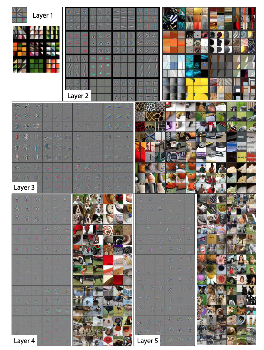
和对卷积层进行简单的成像不同,他们尝试把不同的内容输入到训练好的神经网络,并观察记录卷积核的激活值。并把造成相同卷积核较大激活的内容分组比较。上面的图片中每个九宫格为同一个卷积核对不同图片的聚类。
从上面图片中可以看到,较浅层的卷积层将较为几何抽象的内容归纳到了一起。例如第一层的卷积中,基本就是边缘检测。而在第二层的卷积中,聚类了相似的几何形状,尽管这些几何形状的内容相差甚远。
随着卷积层越来越深,所聚类的内容也越来越具体。例如在第五层里,几乎每个九宫格里都是相同类型的东西。当我们了解这些基础知识后,那么我们有些什么办法可以实现迁移学习?
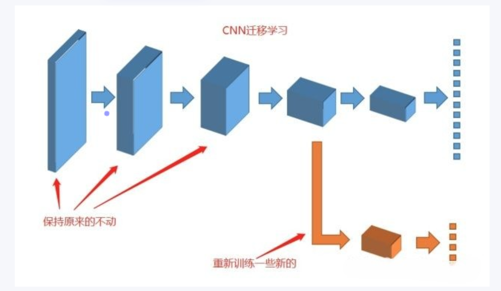
其实有个最简单易行的方式已经摆在我们面前了:如果我们把卷积神经网络的前n层保留下来,剩下不想要的砍掉怎么样?就像我们可以不需要ct能识别狗,识别猫,但是轮廓的对我们还是很有帮助的。
4.2 迁移学习的思想
迁移学习的主要思想是通过利用源任务上学到的特征表示、模型参数或知识,来辅助目标任务的训练过程。这种迁移可以帮助解决以下问题:
- 数据稀缺问题:当目标任务的数据量较少时,通过迁移学习可以利用源任务上丰富的数据信息来提高对目标任务的建模能力和泛化能力。
- 高维输入问题:当目标任务的输入数据具有高维特征时,迁移学习可以借助已经学到的特征表示,减少目标任务中的维度灾难问题,提高处理效率和性能。
- 任务相似性问题:当源任务和目标任务在特征空间或输出空间上存在一定的相似性时,迁移学习可以通过共享模型参数或知识的方式,加速目标任务的学习过程,提升性能。
- 领域适应问题:当源任务和目标任务的数据分布存在一定的差异时,迁移学习可以通过对抗训练、领域自适应等方法,实现在不同领域之间的知识传递和迁移。
总结来说,迁移学习是一种将已经学到的知识和模型从源任务迁移到目标任务的方法。它在机器学习和深度学习中都具有重要意义,可以提高模型的泛化能力、减少训练成本,并更好地应对数据稀缺、高维输入和任务相似性等问题。
4.3 如何使用迁移学习
你可以在自己的预测模型问题上使用迁移学习。以下是两个常用的方法:
- 开发模型的方法
- 预训练模型的方法
开发模型的方法
- 选择源任务。你必须选择一个具有丰富数据的相关的预测建模问题,原任务和目标任务的输入数据、输出数据以及从输入数据和输出数据之间的映射中学到的概念之间有某种关系,
- 开发源模型。然后,你必须为第一个任务开发一个精巧的模型。这个模型一定要比普通的模型更好,以保证一些特征学习可以被执行。
- 重用模型。然后,适用于源任务的模型可以被作为目标任务的学习起点。这可能将会涉及到全部或者部分使用第一个模型,这依赖于所用的建模技术。
- 调整模型。模型可以在目标数据集中的输入-输出对上选择性地进行微调,以让它适应目标任务。
预训练模型方法
- 选择源模型。一个预训练的源模型是从可用模型中挑选出来的。很多研究机构都发布了基于超大数据集的模型,这些都可以作为源模型的备选者。
- 重用模型。选择的预训练模型可以作为用于第二个任务的模型的学习起点。这可能涉及到全部或者部分使用与训练模型,取决于所用的模型训练技术。
- 调整模型。模型可以在目标数据集中的输入-输出对上选择性地进行微调,以让它适应目标任务。
第二种类型的迁移学习在深度学习领域比较常用。
4.4 什么时候使用迁移学习?
迁移学习是一种优化,是一种节省时间或者得到更好性能的捷径。
通常而言,在模型经过开发和测试之前,并不能明显地发现使用迁移学习带来的性能提升。
Lisa Torrey 和 Jude Shavlik 在他们关于迁移学习的章节中描述了使用迁移学习的时候可能带来的三种益处:
- 更高的起点。在微调之前,源模型的初始性能要比不使用迁移学习来的高。
- 更高的斜率。在训练的过程中源模型提升的速率要比不使用迁移学习来得快。
- 更高的渐进。训练得到的模型的收敛性能要比不使用迁移学习更好。
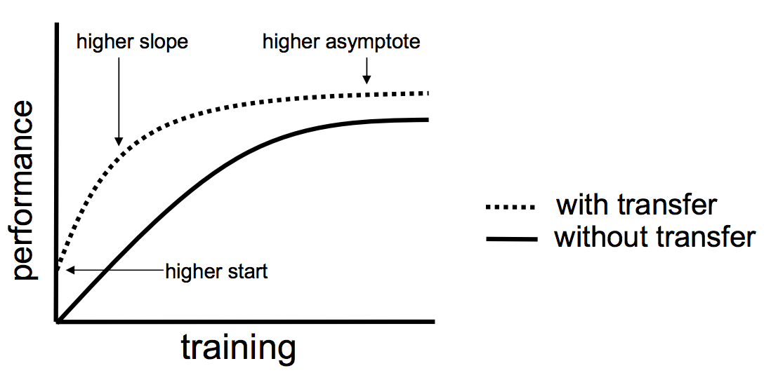
理想情况下,在一个成功的迁移学习应用中,你会得到上述这三种益处。
如果你能够发现一个与你的任务有相关性的任务,它具备丰富的数据,并且你也有资源来为它开发模型,那么,在你的任务中重用这个模型确实是一个好方法,或者(更好的情况),有一个可用的预训练模型,你可以将它作为你自己模型的训练初始点。
在一些问题上,你或许没有那么多的数据,这时候迁移学习可以让你开发出相对不使用迁移学习而言具有更高性能的模型。
简短解读冻结与解冻
一、引言
If I have seen further, it is by standing on the shoulders of giants.
迁移学习在计算机视觉领域中是一种很流行的方法,因为它可以建立精确的模型,耗时更短。利用迁移学习,不是从零开始学习,而是从之前解决各种问题时学到的模式开始。这样,我们就可以利用以前的学习成果,避免从零开始。
二、使用预训练权重
在计算机视觉领域中,迁移学习通常是通过使用预训练模型来表示的。预训练模型是在大型基准数据集上训练的模型,用于解决相似的问题。由于训练这种模型的计算成本较高,因此,导入已发布的成果并使用相应的模型是比较常见的做法。例如,在目标检测任务中,首先要利用主干神经网络进行特征提取,这里使用的backbone一般就是VGG、ResNet等神经网络,因此在训练一个目标检测模型时,可以使用这些神经网络的预训练权重来将backbone的参数初始化,这样在一开始就能提取到比较有效的特征。
可能大家会有疑问,预训练权重是针对他们数据集训练得到的,如果是训练自己的数据集还能用吗?预训练权重对于不同的数据集是通用的,因为特征是通用的。一般来讲,从0开始训练效果会很差,因为权值太过随机,特征提取效果不明显。对于目标检测模型来说,一般不从0开始训练,至少会使用主干部分的权值,虽然有些论文提到了可以不用预训练,但这主要是因为他们的数据集比较大而且他们的调参能力很强。如果从0开始训练,网络在前几个epoch的Loss可能会非常大,并且多次训练得到的训练结果可能相差很大,因为权重初始化太过随机。
PyTorch提供了state_dict()和load_state_dict()两个方法用来保存和加载模型参数,前者将模型参数保存为字典形式,后者将字典形式的模型参数载入到模型当中。下面是使用预训练权重(加载预训练模型)的代码,其中model_path就是预训练权重文件的路径:
# 第一步:读取当前模型参数
model_dict = model.state_dict()
# 第二步:读取预训练模型
pretrained_dict = torch.load(model_path, map_location = device)
pretrained_dict = {

    k: v for k, v in pretrained_dict.items() if np.shape(model_dict[k]) == np.shape(v)}
# 第三步:使用预训练的模型更新当前模型参数
model_dict.update(pretrained_dict)
# 第四步:加载模型参数
model.load_state_dict(model_dict)
但是,使用load_state_dict()加载模型参数时,要求保存的模型参数键值类型和模型完全一致,一旦我们对模型结构做了些许修改,就会出现类似unexpected key module.xxx.weight问题。比如在目标检测模型中,如果修改了主干特征提取网络,只要不是直接替换为现有的其它神经网络,基本上预训练权重是不能用的,要么就自己判断权值里卷积核的shape然后去匹配,要么就只能利用这个主干网络在诸如ImageNet这样的数据集上训练一个自己的预训练模型;如果修改的是后面的neck或者是head的话,前面的backbone的预训练权重还是可以用的。下面是权值匹配的示例代码,把不匹配的直接pass了:
model_dict = model.state_dict()
pretrained_dict = torch.load(model_path, map_location=device)
temp = {}
for k, v in pretrained_dict.items():
    try:
        if np.shape(model_dict[k]) == np.shape(v):
            temp[k]=v
    except:
        pass
model_dict.update(temp)
三、冻结训练
冻结训练其实也是迁移学习的思想,在目标检测任务中用得十分广泛。因为目标检测模型里,主干特征提取部分所提取到的特征是通用的,把backbone冻结起来训练可以加快训练效率,也可以防止权值被破坏。在冻结阶段,模型的主干被冻结了,特征提取网络不发生改变,占用的显存较小,仅对网络进行微调。在解冻阶段,模型的主干不被冻结了,特征提取网络会发生改变,占用的显存较大,网络所有的参数都会发生改变。举个例子,如果在解冻阶段设置batch_size为4,那么在冻结阶段有可能可以把batch_size设置到8。下面是进行冻结训练的示例代码,假设前50个epoch冻结,后50个epoch解冻:
# 冻结阶段训练参数,learning_rate和batch_size可以设置大一点
Init_Epoch          = 0
Freeze_Epoch        = 50
Freeze_batch_size   = 8
Freeze_lr           = 1e-3
# 解冻阶段训练参数,learning_rate和batch_size设置小一点
UnFreeze_Epoch      = 100
Unfreeze_batch_size = 4
Unfreeze_lr         = 1e-4
# 可以加一个变量控制是否进行冻结训练
Freeze_Train        = True
# 冻结一部分进行训练
batch_size  = Freeze_batch_size
lr          = Freeze_lr
start_epoch = Init_Epoch
end_epoch   = Freeze_Epoch
if Freeze_Train:
	for param in model.backbone.parameters():
	param.requires_grad = False
# 解冻后训练
batch_size  = Unfreeze_batch_size
lr          = Unfreeze_lr
start_epoch = Freeze_Epoch
end_epoch   = UnFreeze_Epoch
if Freeze_Train:
	for param in model.backbone.parameters():
	param.requires_grad = True
如果不进行冻结训练,一定要注意参数设置,注意上述代码中冻结阶段和解冻阶段的learning_rate和batch_size是不一样的,另外起始epoch和结束epoch也要重新调整一下。如果是从0开始训练模型(不使用预训练权重),那么一定不能进行冻结训练。
四、预训练和微调
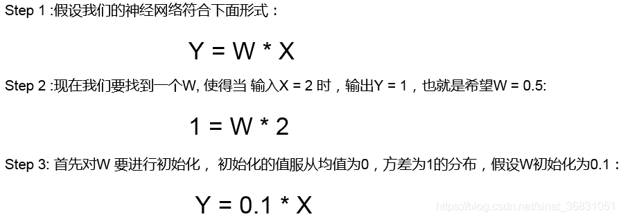
最后再来总结一下预训练和微调,这是两个非常重要的概念,其实也很好理解。举个栗子是最能直观理解的。
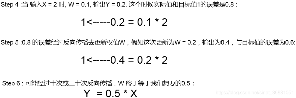
假如我们现在要搭建一个网络模型来完成一个图像分类的任务,首先我们需要把网络的参数进行初始化,然后在训练网络的过程中不断对参数进行调整,直到网络的损失越来越小。在训练过程中,一开始初始化的参数会不断变化,如果结果已经满意了,那我们就可以把训练好的模型参数保存下来,以便训练好的模型可以在下次执行类似任务的时候获得比较好的效果。这个过程就是预训练(Pre-Training)。
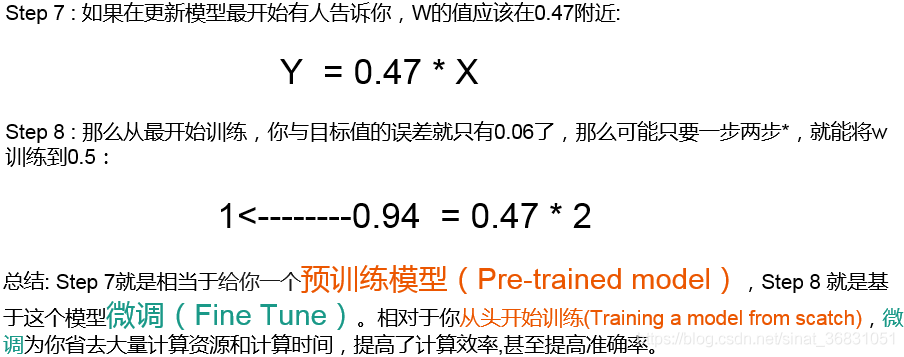
假如在完成上面的模型训练后,我们又接到另一个类似的图像分类任务,这时我们就可以直接使用之前保存下来的模型参数作为这一次任务的初始化参数,然后在训练过程中依据结果不断进行修改,这个过程就是微调(Fine-Tuning)。
我们使用的神经网络越深,就需要越多的样本来进行训练,否则就很容易出现过拟合现象。比如我们想训练一个识别猫的模型,但是自己标注数据精力有限只标了100张,这时就可以考虑ImageNet数据集,可以在ImageNet上训练一个模型,然后使用该模型作为类似任务的初始化或特征提取器,这样既节省了时间和计算资源,又能很快地达到较好的效果。当然,采用预训练+微调也不是绝对有效的,上面识别猫的例子可以这样做是因为ImageNet里有猫的图像,所以可以认为是一个类似的数据集,如果是识别癌细胞的话,效果可能就不是那么好了。关于预训练和微调是有很多策略的,经验也很重要。
对比优化器optimizer与requires_grad冻结
首先,我们知道,深度学习网络中的参数是通过计算梯度,在反向传播进行更新的,从而能得到一个优秀的参数,但是有的时候,我们想固定其中的某些层的参数不参与反向传播。比如说,进行微调时,我们想固定已经加载预训练模型的参数部分,只想更新最后一层的分类器,这时应该怎么做呢。
定义网络
# 定义一个简单的网络
class net(nn.Module):
    def __init__(self, num_class=10):
        super(net, self).__init__()
        self.fc1 = nn.Linear(8, 4)
        self.fc2 = nn.Linear(4, num_class)


    def forward(self, x):
        return self.fc2(self.fc1(x))
情况一:当不冻结层时
代码
model = net()

# 情况一:不冻结参数时
loss_fn = nn.CrossEntropyLoss()
optimizer = optim.SGD(model.parameters(), lr=1e-2)  # 传入的是所有的参数

# 训练前的模型参数
print("model.fc1.weight", model.fc1.weight)
print("model.fc2.weight", model.fc2.weight)

for epoch in range(10):
    x = torch.randn((3, 8))
    label = torch.randint(0,10,[3]).long()
    output = model(x)

    loss = loss_fn(output, label)
    optimizer.zero_grad()
    loss.backward()
    optimizer.step()

# 训练后的模型参数
print("model.fc1.weight", model.fc1.weight)
print("model.fc2.weight", model.fc2.weight)
结果
(bbn) jyzhang@admin2-X10DAi:~/test$ python -u "/home/jyzhang/test/net.py"
model.fc1.weight Parameter containing:
tensor([[ 0.3362, -0.2676, -0.3497, -0.3009, -0.1013, -0.2316, -0.0189,  0.1430],
        [-0.2486,  0.2900, -0.1818, -0.0942,  0.1445,  0.2410, -0.1407, -0.3176],
        [-0.3198,  0.2039, -0.2249,  0.2819, -0.3136, -0.2794, -0.3011, -0.2270],
        [ 0.3376, -0.0842,  0.2747, -0.0232,  0.0768,  0.3160, -0.1185,  0.2911]],
       requires_grad=True)
model.fc2.weight Parameter containing:
tensor([[ 0.4277,  0.0945,  0.1768,  0.3773],
        [-0.4595, -0.2447,  0.4701,  0.2873],
        [ 0.3281, -0.1861, -0.2202,  0.4413],
        [-0.1053, -0.1238,  0.0275, -0.0072],
        [-0.4448, -0.2787, -0.0280,  0.4629],
        [ 0.4063, -0.2091,  0.0706,  0.3216],
        [-0.2287, -0.1352, -0.0502,  0.3434],
        [-0.2946, -0.4074,  0.4926, -0.0832],
        [-0.2608,  0.0165,  0.0501, -0.1673],
        [ 0.2507,  0.3006,  0.0481,  0.2257]], requires_grad=True)
model.fc1.weight Parameter containing:
tensor([[ 0.3316, -0.2628, -0.3391, -0.2989, -0.0981, -0.2178, -0.0056,  0.1410],
        [-0.2529,  0.2991, -0.1772, -0.0992,  0.1447,  0.2480, -0.1370, -0.3186],
        [-0.3246,  0.2055, -0.2229,  0.2745, -0.3158, -0.2750, -0.2994, -0.2295],
        [ 0.3366, -0.0877,  0.2693, -0.0182,  0.0807,  0.3117, -0.1184,  0.2946]],
       requires_grad=True)
model.fc2.weight Parameter containing:
tensor([[ 0.4189,  0.0985,  0.1723,  0.3804],
        [-0.4593, -0.2356,  0.4772,  0.2784],
        [ 0.3269, -0.1874, -0.2173,  0.4407],
        [-0.1061, -0.1248,  0.0309, -0.0062],
        [-0.4322, -0.2868, -0.0319,  0.4647],
        [ 0.4048, -0.2150,  0.0692,  0.3228],
        [-0.2252, -0.1353, -0.0433,  0.3396],
        [-0.2936, -0.4118,  0.4875, -0.0782],
        [-0.2625,  0.0192,  0.0509, -0.1670],
        [ 0.2474,  0.3056,  0.0418,  0.2265]], requires_grad=True)
结论
当不冻结层时,随着训练的进行,模型中的可学习参数层的参数会发生改变
情况二:采用方式一冻结fc1层时
方式一
-
优化器传入所有的参数
optimizer = optim.SGD(model.parameters(), lr=1e-2) # 传入的是所有的参数 -
将要冻结层的参数的
requires_grad置为Falsefor name, param in model.named_parameters(): if "fc1" in name: param.requires_grad = False
代码
# 情况二:采用方式一冻结fc1层时
loss_fn = nn.CrossEntropyLoss()
optimizer = optim.SGD(model.parameters(), lr=1e-2) # 优化器传入的是所有的参数
# 训练前的模型参数
print("model.fc1.weight", model.fc1.weight)
print("model.fc2.weight", model.fc2.weight)
# 冻结fc1层的参数
for name, param in model.named_parameters():
    if "fc1" in name:
        param.requires_grad = False
for epoch in range(10):
x = torch.randn((3, 8))
label = torch.randint(0,10,[3]).long()
output = model(x)
loss = loss_fn(output, label)
optimizer.zero_grad()
loss.backward()
optimizer.step()
print("model.fc1.weight", model.fc1.weight)
print("model.fc2.weight", model.fc2.weight)
结果
(bbn) jyzhang@admin2-X10DAi:~/test$ python -u "/home/jyzhang/test/net.py"
model.fc1.weight Parameter containing:
tensor([[ 0.3163, -0.1592, -0.2360,  0.1436,  0.1158,  0.0406, -0.0627,  0.0566],
        [-0.1688,  0.3519,  0.2464, -0.2693,  0.1284,  0.0544, -0.0188,  0.2404],
        [ 0.0738,  0.2013,  0.0868,  0.1396, -0.2885,  0.3431, -0.1109,  0.2549],
        [ 0.1222, -0.1877,  0.3511,  0.1951,  0.2147, -0.0427, -0.3374, -0.0653]],
       requires_grad=True)
model.fc2.weight Parameter containing:
tensor([[-0.1830, -0.3147, -0.1698,  0.3235],
        [-0.1347,  0.3096,  0.4895,  0.1221],
        [ 0.2735, -0.2238,  0.4713, -0.0683],
        [-0.3150, -0.1905,  0.3645,  0.3766],
        [-0.0340,  0.3212,  0.0650,  0.1380],
        [-0.2500,  0.1128, -0.3338, -0.4151],
        [ 0.0446, -0.4776, -0.3655,  0.0822],
        [-0.1871, -0.0602, -0.4855, -0.3604],
        [-0.3296,  0.0523, -0.3424,  0.2151],
        [-0.2478,  0.1424,  0.4547, -0.1969]], requires_grad=True)
model.fc1.weight Parameter containing:
tensor([[ 0.3163, -0.1592, -0.2360,  0.1436,  0.1158,  0.0406, -0.0627,  0.0566],
        [-0.1688,  0.3519,  0.2464, -0.2693,  0.1284,  0.0544, -0.0188,  0.2404],
        [ 0.0738,  0.2013,  0.0868,  0.1396, -0.2885,  0.3431, -0.1109,  0.2549],
        [ 0.1222, -0.1877,  0.3511,  0.1951,  0.2147, -0.0427, -0.3374, -0.0653]])
model.fc2.weight Parameter containing:
tensor([[-0.1821, -0.3155, -0.1637,  0.3213],
        [-0.1353,  0.3130,  0.4807,  0.1245],
        [ 0.2731, -0.2206,  0.4687, -0.0718],
        [-0.3138, -0.1925,  0.3561,  0.3809],
        [-0.0344,  0.3152,  0.0606,  0.1332],
        [-0.2501,  0.1154, -0.3267, -0.4137],
        [ 0.0400, -0.4723, -0.3586,  0.0808],
        [-0.1823, -0.0667, -0.4854, -0.3543],
        [-0.3285,  0.0547, -0.3388,  0.2166],
        [-0.2497,  0.1410,  0.4551, -0.2008]], requires_grad=True)
结论
由实验的结果可以看出:只要设置requires_grad=False虽然传入模型所有的参数,仍然只更新requires_grad=True的层的参数
情况三:采用方式二冻结fc1层时
方式二
-
优化器传入不冻结的fc2层的参数
optimizer = optim.SGD(model.fc2.parameters(), lr=1e-2) # 优化器只传入fc2的参数 -
注:不需要将要冻结层的参数的
requires_grad置为False
代码
# 情况三:采用方式二冻结fc1层时
loss_fn = nn.CrossEntropyLoss()
optimizer = optim.SGD(model.fc2.parameters(), lr=1e-2)  # 优化器只传入fc2的参数
print("model.fc1.weight", model.fc1.weight)
print("model.fc2.weight", model.fc2.weight)

for epoch in range(10):
    x = torch.randn((3, 8))
    label = torch.randint(0,3,[3]).long()
    output = model(x)

    loss = loss_fn(output, label)
    optimizer.zero_grad()
    loss.backward()
    optimizer.step()

print("model.fc1.weight", model.fc1.weight)
print("model.fc2.weight", model.fc2.weight)
结果
model.fc1.weight Parameter containing:
tensor([[ 0.2519, -0.1772, -0.2229,  0.0711, -0.1681,  0.1233, -0.3217, -0.0412],
        [ 0.2032, -0.2045,  0.2723,  0.3272,  0.1034,  0.1519, -0.0587, -0.3436],
        [ 0.0470,  0.2379,  0.0590,  0.2400,  0.2280,  0.2045, -0.0229, -0.3484],
        [-0.3023, -0.1195,  0.1792, -0.2173, -0.0492,  0.2640, -0.3511, -0.2845]],
       requires_grad=True)
model.fc2.weight Parameter containing:
tensor([[-0.3263, -0.2938, -0.3516, -0.4578],
        [-0.4549, -0.0060,  0.4696, -0.0174],
        [-0.4841,  0.2861,  0.2658,  0.4483],
        [-0.3093,  0.0977, -0.2735,  0.1033],
        [-0.2421,  0.4489, -0.4649,  0.0110],
        [-0.3671,  0.0182, -0.1027, -0.4441],
        [ 0.0205, -0.0659,  0.4183, -0.2068],
        [-0.1846,  0.1741, -0.2302, -0.1745],
        [-0.3423, -0.2642,  0.2796,  0.4976],
        [-0.0770, -0.3766, -0.0512, -0.2105]], requires_grad=True)
model.fc1.weight Parameter containing:
tensor([[ 0.2519, -0.1772, -0.2229,  0.0711, -0.1681,  0.1233, -0.3217, -0.0412],
        [ 0.2032, -0.2045,  0.2723,  0.3272,  0.1034,  0.1519, -0.0587, -0.3436],
        [ 0.0470,  0.2379,  0.0590,  0.2400,  0.2280,  0.2045, -0.0229, -0.3484],
        [-0.3023, -0.1195,  0.1792, -0.2173, -0.0492,  0.2640, -0.3511, -0.2845]],
       requires_grad=True)
model.fc2.weight Parameter containing:
tensor([[-0.3253, -0.2973, -0.3707, -0.4560],
        [-0.4566,  0.0015,  0.4655, -0.0166],
        [-0.4796,  0.2931,  0.2592,  0.4661],
        [-0.3097,  0.0966, -0.2695,  0.1002],
        [-0.2433,  0.4455, -0.4587,  0.0063],
        [-0.3669,  0.0171, -0.0988, -0.4452],
        [ 0.0198, -0.0679,  0.4203, -0.2088],
        [-0.1854,  0.1717, -0.2241, -0.1781],
        [-0.3429, -0.2653,  0.2822,  0.4938],
        [-0.0773, -0.3765, -0.0464, -0.2127]], requires_grad=True)
结论
当优化器只传入要更新的层的参数时,只会更新优化器传入的参数,对于没有传入的参数可以求导,但是仍然不会更新参数
方式一与方式二对比总结
在训练过程中可能需要固定一部分模型的参数,只更新另一部分参数。
有两种思路实现这个目标,一个是设置不要更新参数的网络层为false,另一个就是在定义优化器时只传入要更新的参数。
最优做法是,优化器只传入requires_grad=True的参数,这样占用的内存会更小一点,效率也会更高。
最优写法
最优写法
将不更新的参数的requires_grad设置为False,同时不将该参数传入optimizer
-
将不更新的参数的
requires_grad设置为False# 冻结fc1层的参数 for name, param in model.named_parameters(): if "fc1" in name: param.requires_grad = False -
不将不更新的模型参数传入
optimizer# 定义一个fliter,只传入requires_grad=True的模型参数 optimizer = optim.SGD(filter(lambda p : p.requires_grad, model.parameters()), lr=1e-2)
代码
# 最优写法
loss_fn = nn.CrossEntropyLoss()
# # 训练前的模型参数
print("model.fc1.weight", model.fc1.weight)
print("model.fc2.weight", model.fc2.weight)
print("model.fc1.weight.requires_grad:", model.fc1.weight.requires_grad)
print("model.fc2.weight.requires_grad:", model.fc2.weight.requires_grad)
# 冻结fc1层的参数
for name, param in model.named_parameters():
    if "fc1" in name:
        param.requires_grad = False
optimizer = optim.SGD(filter(lambda p : p.requires_grad, model.parameters()), lr=1e-2) # 定义一个fliter,只传入requires_grad=True的模型参数
for epoch in range(10):
x = torch.randn((3, 8))
label = torch.randint(0,3,[3]).long()
output = model(x)
loss = loss_fn(output, label)
optimizer.zero_grad()
loss.backward()
optimizer.step()
print("model.fc1.weight", model.fc1.weight)
print("model.fc2.weight", model.fc2.weight)
print("model.fc1.weight.requires_grad:", model.fc1.weight.requires_grad)
print("model.fc2.weight.requires_grad:", model.fc2.weight.requires_grad)
结果
(bbn) jyzhang@admin2-X10DAi:~/test$ python -u "/home/jyzhang/test/net.py"
model.fc1.weight Parameter containing:
tensor([[-0.1193,  0.2354,  0.2520,  0.1187,  0.2699, -0.2301,  0.1622, -0.0478],
        [-0.2862, -0.1716,  0.2865,  0.2615, -0.2205, -0.2046, -0.0983, -0.1564],
        [-0.3143, -0.2248,  0.2198,  0.2338,  0.1184, -0.2033, -0.3418,  0.1434],
        [ 0.3107, -0.0411, -0.3016,  0.1924, -0.1756, -0.2881,  0.0528, -0.0444]],
       requires_grad=True)
model.fc2.weight Parameter containing:
tensor([[-0.2548,  0.2107, -0.1293, -0.2562],
        [-0.1989, -0.2624,  0.2226,  0.4861],
        [-0.1501,  0.2516,  0.4311, -0.1650],
        [ 0.0334, -0.0963, -0.1731,  0.1706],
        [ 0.2451, -0.2102,  0.0499,  0.0497],
        [-0.1464, -0.2973,  0.3692,  0.0523],
        [ 0.1192,  0.3575, -0.1911,  0.1457],
        [-0.0990,  0.2059,  0.2072, -0.2013],
        [-0.4397,  0.4036, -0.3402, -0.0417],
        [ 0.0379,  0.0128, -0.3212, -0.0867]], requires_grad=True)
model.fc1.weight.requires_grad: True
model.fc2.weight.requires_grad: True
model.fc1.weight Parameter containing:
tensor([[-0.1193,  0.2354,  0.2520,  0.1187,  0.2699, -0.2301,  0.1622, -0.0478],
        [-0.2862, -0.1716,  0.2865,  0.2615, -0.2205, -0.2046, -0.0983, -0.1564],
        [-0.3143, -0.2248,  0.2198,  0.2338,  0.1184, -0.2033, -0.3418,  0.1434],
        [ 0.3107, -0.0411, -0.3016,  0.1924, -0.1756, -0.2881,  0.0528, -0.0444]])
model.fc2.weight Parameter containing:
tensor([[-0.2637,  0.2073, -0.1293, -0.2422],
        [-0.2027, -0.2641,  0.2152,  0.4897],
        [-0.1543,  0.2504,  0.4188, -0.1576],
        [ 0.0356, -0.0947, -0.1698,  0.1669],
        [ 0.2474, -0.2081,  0.0536,  0.0456],
        [-0.1445, -0.2962,  0.3708,  0.0500],
        [ 0.1219,  0.3574, -0.1876,  0.1404],
        [-0.0961,  0.2058,  0.2091, -0.2046],
        [-0.4368,  0.4039, -0.3376, -0.0450],
        [ 0.0398,  0.0143, -0.3181, -0.0897]], requires_grad=True)
model.fc1.weight.requires_grad: False
model.fc2.weight.requires_grad: True
结论
最优写法能够节省显存和提升速度:
- 节省显存:不将不更新的参数传入
optimizer - 提升速度:将不更新的参数的
requires_grad设置为False,节省了计算这部分参数梯度的时间
一些重要的代码总结
 # 冻结network1的全部参数和network2的部分参数
 for name, parameter in network1.named_parameters():
     parameter.requires_grad = False

 for name, parameter in network2.named_parameters():
     if 'key' in name:
         parameter.requires_grad = False

# 优化器中过滤filter冻结的参数
optimizer_network2 = torch.optim.Adam(filter(lambda p: p.requires_grad, network2.parameters()), lr=0.005, betas=(0.5, 0.999))
# 结合加载模型部分参数的情况,优化器需要按如下设置:
optimizer_network2 = torch.optim.Adam([{

    'params': filter(lambda p: p.requires_grad, network2.parameters()), 'initial_lr': 0.0002}], lr=0.005, betas=(0.5, 0.999))
for p in self.backbone.parameters():
    p.requires_grad = False

class classifer(nn.Module):
	def __init__(self,in_ch,num_classes):
		super().__init__()
		self.avgpool = nn.AdaptiveAvgPool1d(1)
		self.fc = nn.Linear(in_ch,num_classes)

	def forward(self, x):
		x = self.avgpool(x.transpose(1, 2))  # B C 1
		x = torch.flatten(x, 1)
		x = self.fc(x)
		return x

class Swin(nn.Module):
    def __init__(self):
        super().__init__()
        #创建模型,并且加载预训练参数
        self.swin= create_model('swin_large_patch4_window7_224_in22k',pretrained=True)
        #整体模型的结构
        pretrained_dict = self.swin.state_dict()
        #去除模型的分类层
        self.backbone = nn.Sequential(*list(self.swin.children())[:-2])
        #去除分类层的模型架构
        model_dict = self.backbone.state_dict()

        # 将pretrained_dict里不属于model_dict的键剔除掉
        pretrained_dict = {

    k: v for k, v in pretrained_dict.items() if k in model_dict}
        # 更新现有的model_dict
        model_dict.update(pretrained_dict)
        # 加载我们真正需要的state_dict
        self.backbone.load_state_dict(model_dict)
        #屏蔽除分类层所有的参数
        for p in self.backbone.parameters():
            p.requires_grad = False
        #构建新的分类层
        self.head = classifer(1536, 14)

    def forward(self, x):
        x = self.backbone(x)
        x=self.head(x)
        return x

optimizer = torch.optim.Adam(filter(lambda p: p.requires_grad, cnn.parameters()), lr=1e-4, betas=(0.9, 0.999),weight_decay=1e-6)

if epoch ==1:
    for p in  Swin.backbone.parameters():
        p.requires_grad = True
        optimizer.add_param_group({

    'params': Swin.backbone.parameters()})
# we want to freeze the fc2 layer this time: only train fc1 and fc3
net.fc2.weight.requires_grad = False
net.fc2.bias.requires_grad = False

# passing only those parameters that explicitly requires grad
optimizer = optim.Adam(filter(lambda p: p.requires_grad, net.parameters()), lr=0.1)

# then do the normal execution of loss calculation and backward propagation

#  unfreezing the fc2 layer for extra tuning if needed
net.fc2.weight.requires_grad = True
net.fc2.bias.requires_grad = True

# add the unfrozen fc2 weight to the current optimizer
optimizer.add_param_group({

    'params': net.fc2.parameters()})

if self.frozen_pretrained_weights:
  self.eval()
    with torch.no_grad():
      output = self.encoders(batch)
  else:
    output = self.encoders(batch)
# 这将冻结 Resnet50 总共 10 层中的第 1-6 层。希望这有帮助!
model_ft = models.resnet50(pretrained=True)
ct = 0
for child in model_ft.children():
ct += 1
if ct < 7:
    for param in child.parameters():
        param.requires_grad = False
# let's unfreeze the fc2 layer this time for extra tuning
net.fc2.weight.requires_grad = True
net.fc2.bias.requires_grad = True

# add the unfrozen fc2 weight to the current optimizer
optimizer.add_param_group({

    'params': net.fc2.parameters()})
def dfs_freeze(model):
    for name, child in model.named_children():
        for param in child.parameters():
            param.requires_grad = False
        dfs_freeze(child)
optimizer = torch.optim.Adam(filter(lambda p: p.requires_grad, model.parameters()), lr=opt.lr, amsgrad=True)
预训练模型与自己模型参数不匹配和模型微调
导入预训练模型在通常情况下都能加快模型收敛,提升模型性能。但根据实际任务需求,自己搭建的模型往往和通用的Backbone并不能做到网络层的完全一致,无非就是少一些层和多一些层两种情况。
1. 自己模型层数较少
net = ...   # net为自己的模型
save_model = torch.load('path_of_pretrained_model') # 获取预训练模型字典(键值对)
model_dict = net.state_dict() # 获取自己模型字典(键值对)
# 新定义字典,用来获取自己模型中对应层的预训练模型中的参数
state_dict = {

    k:v for k,v in save_model.items() if k in model_dict.keys()}
model_dict.update(state_dict) # 更新自己模型字典中键值对
net.load_state_dict(model_dict) # 加载参数
其中update:对于state_dict和model_dict都有的键值对,前者对应的值会替换后者,若前者有后者没有的键值对,则会添加这些键值对到后者字典中。
2. 自己模型层数较多
model_dict = model.state_dict() # 自己模型字典
model_dict.update(pretrained_model) # 直接将预训练模型参数更新进来
model.load_state_dict(model_dict) # 加载
结果与预训练模型对应的层权重被加载了,其它层则为默认初始化。
由于模型参数都为字典形式存在,可以用字典的增删方式进行更灵活的操作
特征提取与微调
迁移学习是一种有效的机器学习方法,尤其是在数据不足的情况下。它通过使用在大型数据集(如 ImageNet)上预训练的模型,将这些模型的知识应用于新的、相对较小的数据集上。下面,我将详细解释两种主要的迁移学习策略,并提供相应的代码示例。
1. 特征提取(Feature Extraction)
在这种策略中,你使用预训练模型的卷积层(即模型的前几层)来作为固定的特征提取器。然后,你只需添加一些新的可训练层(通常是全连接层),以便根据新的数据集进行预测。
代码示例
假设我们要在一个新的数据集上使用预训练的 ResNet 模型进行特征提取:
import torch
import torch.nn as nn
from torchvision import models

# 加载预训练的 ResNet 模型
model = models.resnet18(pretrained=True)
# 冻结所有卷积层的参数
for param in model.parameters():
    param.requires_grad = False

# 替换最后的全连接层
num_ftrs = model.fc.in_features
model.fc = nn.Linear(num_ftrs, 2) # 假设我们的新数据集有2个类别
# 现在,只有 model.fc 层的参数会在训练中更新
在这个示例中,我们首先加载了预训练的 ResNet 模型,并冻结了它的所有卷积层。然后,我们替换了最后的全连接层以适应新的分类任务(假设有两个类别)。在训练过程中,只有这个新添加的全连接层的参数会更新。
2. 微调(Fine-Tuning)
微调涉及到在预训练模型的基础上进一步训练整个模型(或模型的大部分层)。这通常是在特征提取的基础上进行的,即首先使用特征提取策略训练模型,然后解冻整个模型的多个层,并对整个模型进行进一步的训练。
代码示例
继续使用上面的 ResNet 示例,我们现在将进行微调:
# 之前的代码省略...
# 解冻所有层
for param in model.parameters():
    param.requires_grad = True
# 现在整个模型的参数都会在训练中更新
在微调阶段,所有层的参数都会被更新。这通常是在特征提取阶段之后进行,特别是当新数据集与原始数据集在特征上有较大差异时。
添加、删除或修改字典中的项
在 PyTorch 中,模型的参数是以字典形式存储的,这使得我们可以利用 Python 字典的特性来灵活地处理模型参数。例如,我们可以添加、删除或修改字典中的项,以此来自定义模型的参数。以下是一些常见操作的示例:
修改
示例:修改特定层的参数
假设您想要修改预训练模型中某一层的参数,比如将第一层卷积层的权重全部设置为零。
import torch
import torchvision.models as models

# 加载预训练模型
model = models.resnet18(pretrained=True)
# 将第一层卷积层的权重设置为零
torch.nn.init.constant_(model.conv1.weight, 0)
在这个示例中,我们使用 torch.nn.init.constant_ 方法直接修改了模型的第一层卷积层(conv1)的权重,将其全部设置为零。
示例:修改层的属性
除了修改层的参数外,您还可以修改层的其他属性。例如,您可能想要更改卷积层的步长(stride)或填充(padding)。
# 改变第一层卷积层的步长和填充
model.conv1.stride = (2, 2)
model.conv1.padding = (1, 1)
在这个示例中,我们修改了模型的第一层卷积层的步长和填充属性。
注意事项
- 在修改模型的参数或属性时,请确保您的修改不会导致模型架构的不一致。例如,更改卷积层的核大小或步长可能会影响模型中后续层的输入尺寸。
- 修改模型参数通常需要对模型的工作原理有深入的理解,以避免意外地破坏模型的性能。
通过这些修改,您可以对模型进行微调,使其更好地适应特定的任务或数据集。这种能力在进行模型实验和优化时非常有价值。
示例 1:删除特定层的参数
假设你想要从预训练模型中删除某些层的参数。这可以通过删除字典中相应的键值对来实现。
import torch
import torchvision.models as models

# 加载预训练模型
model = models.resnet18(pretrained=True)

# 获取模型的 state_dict
model_dict = model.state_dict()

# 假设我们想要删除第一层卷积层的参数
del model_dict['conv1.weight']
del model_dict['conv1.bias']

# 更新模型的 state_dict
model.load_state_dict(model_dict, strict=False)
在这个示例中,我们首先加载了预训练的 ResNet18 模型,并获取其状态字典。然后,我们删除了第一层卷积层(conv1)的权重和偏置参数。最后,我们使用 load_state_dict 更新模型的参数,strict=False 表示我们允许不匹配的项存在。
示例 2:添加新层的参数
如果你想向模型中添加新的层,并为其初始化参数,可以直接向状态字典中添加新的键值对。
import torch.nn as nn

# 继续之前的模型
# 添加一个新的全连接层
num_ftrs = model.fc.in_features
model.fc = nn.Sequential(
               nn.Linear(num_ftrs, 500),
               nn.ReLU(),
               nn.Linear(500, 2)
           )

# 初始化新层的参数
nn.init.xavier_normal_(model.fc[0].weight)
nn.init.constant_(model.fc[0].bias, 0)
nn.init.xavier_normal_(model.fc[2].weight)
nn.init.constant_(model.fc[2].bias, 0)

# 获取新的模型 state_dict
new_model_dict = model.state_dict()

# 可以选择性地将新的 state_dict 保存下来
# torch.save(new_model_dict, 'modified_model.pth')
PyTorch断点训练
主要有以下几方面的内容:
- 对于多步长训练需要保存lr_schedule
- 初始化随机数种子
- 保存每一代最好的结果
简单介绍
最近在尝试用CIFAR10训练分类问题的时候,由于数据集体量比较大,训练的过程中时间比较长,有时候想给停下来,但是停下来了之后就得重新训练,我们学习断点继续训练及继续训练的时候注意epoch的改变等。
Epoch:  9 | train loss: 0.3517 | test accuracy: 0.7184 | train time: 14215.1018  s
Epoch:  9 | train loss: 0.2471 | test accuracy: 0.7252 | train time: 14309.1216  s
Epoch:  9 | train loss: 0.4335 | test accuracy: 0.7201 | train time: 14403.2398  s
Epoch:  9 | train loss: 0.2186 | test accuracy: 0.7242 | train time: 14497.1921  s
Epoch:  9 | train loss: 0.2127 | test accuracy: 0.7196 | train time: 14591.4974  s
Epoch:  9 | train loss: 0.1624 | test accuracy: 0.7142 | train time: 14685.7034  s
Epoch:  9 | train loss: 0.1795 | test accuracy: 0.7170 | train time: 14780.2831  s
绝望!!!!!训练到了一定次数发现训练次数少了,或者中途断了又得重新开始训练
一、模型的保存与加载
PyTorch中的保存(序列化,从内存到硬盘)与反序列化(加载,从硬盘到内存)
torch.save主要参数: obj:对象 、f:输出路径
torch.load 主要参数 :f:文件路径 、map_location:指定存放位置、 cpu or gpu
模型的保存的两种方法:
1、保存整个Module
torch.save(net, path)
2、保存模型参数
state_dict = net.state_dict()
torch.save(state_dict , path)
二、模型的训练过程中保存
checkpoint = {
        "net": model.state_dict(),
        'optimizer':optimizer.state_dict(),
        "epoch": epoch
    }
将网络训练过程中的网络的权重,优化器的权重保存,以及epoch 保存,便于继续训练恢复
在训练过程中,可以根据自己的需要,每多少代,或者多少epoch保存一次网络参数,便于恢复,提高程序的鲁棒性。
checkpoint = {
        "net": model.state_dict(),
        'optimizer':optimizer.state_dict(),
        "epoch": epoch
    }
    if not os.path.isdir("./models/checkpoint"):
        os.mkdir("./models/checkpoint")
    torch.save(checkpoint, './models/checkpoint/ckpt_best_%s.pth' %(str(epoch)))
通过上述的过程可以在训练过程自动在指定位置创建文件夹,并保存断点文件

三、模型的断点继续训练
if RESUME:
    path_checkpoint = "./models/checkpoint/ckpt_best_1.pth"  # 断点路径
    checkpoint = torch.load(path_checkpoint)  # 加载断点

    model.load_state_dict(checkpoint['net'])  # 加载模型可学习参数

    optimizer.load_state_dict(checkpoint['optimizer'])  # 加载优化器参数
    start_epoch = checkpoint['epoch']  # 设置开始的epoch
指出这里的是否继续训练,及训练的checkpoint的文件位置等可以通过argparse从命令行直接读取,也可以通过log文件直接加载,也可以自己在代码中进行修改。关于argparse参照我的这一篇文章:
四、重点在于epoch的恢复
start_epoch = -1


if RESUME:
    path_checkpoint = "./models/checkpoint/ckpt_best_1.pth"  # 断点路径
    checkpoint = torch.load(path_checkpoint)  # 加载断点

    model.load_state_dict(checkpoint['net'])  # 加载模型可学习参数

    optimizer.load_state_dict(checkpoint['optimizer'])  # 加载优化器参数
    start_epoch = checkpoint['epoch']  # 设置开始的epoch


for epoch in  range(start_epoch + 1 ,EPOCH):
    # print('EPOCH:',epoch)
    for step, (b_img,b_label) in enumerate(train_loader):
        train_output = model(b_img)
        loss = loss_func(train_output,b_label)
        # losses.append(loss)
        optimizer.zero_grad()
        loss.backward()
        optimizer.step()
通过定义start_epoch变量来保证继续训练的时候epoch不会变化

一、初始化随机数种子
import torch
import random
import numpy as np

def set_random_seed(seed = 10,deterministic=False,benchmark=False):
    random.seed(seed)
    np.random(seed)
    torch.manual_seed(seed)
    torch.cuda.manual_seed_all(seed)
    if deterministic:
        torch.backends.cudnn.deterministic = True
    if benchmark:
        torch.backends.cudnn.benchmark = True
关于torch.backends.cudnn.deterministic和torch.backends.cudnn.benchmark详见
benchmark用在输入尺寸一致,可以加速训练,deterministic用来固定内部随机性
二、多步长SGD继续训练
在简单的任务中,我们使用固定步长(也就是学习率LR)进行训练,但是如果学习率lr设置的过小的话,则会导致很难收敛,如果学习率很大的时候,就会导致在最小值附近,总会错过最小值,loss产生震荡,无法收敛。所以这要求我们要对于不同的训练阶段使用不同的学习率,一方面可以加快训练的过程,另一方面可以加快网络收敛。
采用多步长 torch.optim.lr_scheduler的多种步长设置方式来实现步长的控制,lr_scheduler的各种使用推荐参考如下教程:
所以我们在保存网络中的训练的参数的过程中,还需要保存lr_scheduler的state_dict,然后断点继续训练的时候恢复
#这里我设置了不同的epoch对应不同的学习率衰减,在10->20->30,学习率依次衰减为原来的0.1,即一个数量级
lr_schedule = torch.optim.lr_scheduler.MultiStepLR(optimizer,milestones=[10,20,30,40,50],gamma=0.1)
optimizer = torch.optim.SGD(model.parameters(),lr=0.1)

for epoch in range(start_epoch+1,80):
    optimizer.zero_grad()
    optimizer.step()
    lr_schedule.step()

    if epoch %10 ==0:
        print('epoch:',epoch)
        print('learning rate:',optimizer.state_dict()['param_groups'][0]['lr'])
lr的变化过程如下:
epoch: 10
learning rate: 0.1
epoch: 20
learning rate: 0.010000000000000002
epoch: 30
learning rate: 0.0010000000000000002
epoch: 40
learning rate: 0.00010000000000000003
epoch: 50
learning rate: 1.0000000000000004e-05
epoch: 60
learning rate: 1.0000000000000004e-06
epoch: 70
learning rate: 1.0000000000000004e-06
我们在保存的时候,也需要对lr_scheduler的state_dict进行保存,断点继续训练的时候也需要恢复lr_scheduler
#加载恢复
if RESUME:
    path_checkpoint = "./model_parameter/test/ckpt_best_50.pth"  # 断点路径
    checkpoint = torch.load(path_checkpoint)  # 加载断点

    model.load_state_dict(checkpoint['net'])  # 加载模型可学习参数

    optimizer.load_state_dict(checkpoint['optimizer'])  # 加载优化器参数
    start_epoch = checkpoint['epoch']  # 设置开始的epoch
    lr_schedule.load_state_dict(checkpoint['lr_schedule'])#加载lr_scheduler


#保存
for epoch in range(start_epoch+1,80):

    optimizer.zero_grad()

    optimizer.step()
    lr_schedule.step()


    if epoch %10 ==0:
        print('epoch:',epoch)
        print('learning rate:',optimizer.state_dict()['param_groups'][0]['lr'])
        checkpoint = {
            "net": model.state_dict(),
            'optimizer': optimizer.state_dict(),
            "epoch": epoch,
            'lr_schedule': lr_schedule.state_dict()
        }
        if not os.path.isdir("./model_parameter/test"):
            os.mkdir("./model_parameter/test")
        torch.save(checkpoint, './model_parameter/test/ckpt_best_%s.pth' % (str(epoch)))
三、保存最好的结果
每一个epoch中的每个step会有不同的结果,可以保存每一代最好的结果,用于后续的训练
第一次实验代码
RESUME = True

EPOCH = 40
LR = 0.0005


model = cifar10_cnn.CIFAR10_CNN()

print(model)
optimizer = torch.optim.Adam(model.parameters(),lr=LR)
loss_func = nn.CrossEntropyLoss()

start_epoch = -1


if RESUME:
    path_checkpoint = "./models/checkpoint/ckpt_best_1.pth"  # 断点路径
    checkpoint = torch.load(path_checkpoint)  # 加载断点

    model.load_state_dict(checkpoint['net'])  # 加载模型可学习参数

    optimizer.load_state_dict(checkpoint['optimizer'])  # 加载优化器参数
    start_epoch = checkpoint['epoch']  # 设置开始的epoch


for epoch in  range(start_epoch + 1 ,EPOCH):
    # print('EPOCH:',epoch)
    for step, (b_img,b_label) in enumerate(train_loader):
        train_output = model(b_img)
        loss = loss_func(train_output,b_label)
        # losses.append(loss)
        optimizer.zero_grad()
        loss.backward()
        optimizer.step()

        if step % 100 == 0:
            now = time.time()
            print('EPOCH:',epoch,'| step :',step,'| loss :',loss.data.numpy(),'| train time: %.4f'%(now-start_time))

    checkpoint = {
        "net": model.state_dict(),
        'optimizer':optimizer.state_dict(),
        "epoch": epoch
    }
    if not os.path.isdir("./models/checkpoint"):
        os.mkdir("./models/checkpoint")
    torch.save(checkpoint, './models/checkpoint/ckpt_best_%s.pth' %(str(epoch)))
更新实验代码
optimizer = torch.optim.SGD(model.parameters(),lr=0.1)
lr_schedule = torch.optim.lr_scheduler.MultiStepLR(optimizer,milestones=[10,20,30,40,50],gamma=0.1)
start_epoch = 9
# print(schedule)


if RESUME:
    path_checkpoint = "./model_parameter/test/ckpt_best_50.pth"  # 断点路径
    checkpoint = torch.load(path_checkpoint)  # 加载断点

    model.load_state_dict(checkpoint['net'])  # 加载模型可学习参数

    optimizer.load_state_dict(checkpoint['optimizer'])  # 加载优化器参数
    start_epoch = checkpoint['epoch']  # 设置开始的epoch
    lr_schedule.load_state_dict(checkpoint['lr_schedule'])

for epoch in range(start_epoch+1,80):

    optimizer.zero_grad()

    optimizer.step()
    lr_schedule.step()


    if epoch %10 ==0:
        print('epoch:',epoch)
        print('learning rate:',optimizer.state_dict()['param_groups'][0]['lr'])
        checkpoint = {


            "net": model.state_dict(),
            'optimizer': optimizer.state_dict(),
            "epoch": epoch,
            'lr_schedule': lr_schedule.state_dict()
        }
        if not os.path.isdir("./model_parameter/test"):
            os.mkdir("./model_parameter/test")
        torch.save(checkpoint, './model_parameter/test/ckpt_best_%s.pth' % (str(epoch)))
深入解读
如果我们的模型训练到一半因为各种原因中断了,重新训练的话之前就白做了,对于需要训练好几天的模型,这显然无法让人接受。那么该如何重新加载模型继续训练呢?这就是断点续训。
常用代码及注意事项
首先我们要训练模型,代码中需先进行以下几个定义:
# 1.定义模型
self.model = CNN()
self.model.to(device)
# 2.定义损失函数
self.criterion = nn.CrossEntropyLoss()
# 3.定义优化器
self.optimizer = optim.Adam(model.parameters(), #可迭代的参数优化或dicts定义
		    lr=1e-3, # 学习率(默认1e-3)
		    betas=(0.9, 0.999), # 用于计算的系数梯度及其平方的运行平均值
		    eps=1e-8, # 增加分母项以提高数值稳定性
		    weight_decay=1e-4, # 权重衰减
            amsgrad=False # 是否使用“Adam and Beyond收敛”一文中该算法的AMSGrad变体`,默认False
            )
# 4.定义动态调整学习率(可不做)
self.lr_scheduler = WarmupMultiStepLR(optimizer=optimizer,
                                     milestones=[100, 300],
                                     gamma=0.1,
                                     warmup_factor=0.1,
                                     warmup_iters=2,
                                     warmup_method="linear",
                                     last_epoch=-1)
注意,model.to(device)将model放入cuda中,这一步一定要在定义optimizer之前做。
训练迭代例子:
self.start_epoch = 0
for self.epoch in range(self.start_epoch, 400):
    for input, target in self.dataset:
        self.optimizer.zero_grad()
        output = self.model(input)
        loss = self.criterion(output, target)
        loss.backward()
        self.optimizer.step()
    self.lr_scheduler.step()
注意,optimizer.step()通常在每个batch之中,而lr_scheduler.step()通常在每个epoch之中。
原因:
step()可看做“每次调用才更新一次”。
所以为了在每个batch中loss反向传播能更新模型,optimizer.step()要紧跟在loss.backward()之后,否则模型不会在每个batch里都更新。
由于动态调整学习率如MutiStepLR、CosineAnnealingLR等,通常都设置成随着epoch变化而变化,所以lr_scheduler.step()要放在每个epoch下,如果也放在每个batch下的话,lr_scheduler将会更新epoch num * batch num次。
之前就是因为不小心把lr_scheduler.step()放在了batch里,导致动态调整学习率没起作用,因为前2个epoch就直接将lr调整到设定的最小值了…
训练状态保存
可以在每次best的时候保存模型状态,或者每个epoch之后都保存。
①主要是保存模型参数、optimizer、lr_scheduler、当前epoch、当前最好的结果best_metric。
import os
import glob.glob as glob

self.best_metric = 0.
# 保存最好的模型
def saveBestWeights(self):
	if self.current_metric >= self.best_metric:
		self.best_metric = self.current_metric
		print('best and save')
		torch.save({

    'epoch': self.epoch, 'state_dict': self.model.state_dict(),
					'optimizer': self.optimizer.state_dict(),
					'scheduler': self.lr_scheduler.state_dict(), 'best_acc': self.best_metric}
				   , os.path.join(self.checkpoint_dir, 'backbone_best.pth'))
# 每次都保存模型
def saveWeights(self, clean_previous=True):
	if clean_previous:
		files = glob(os.path.join(self.checkpoint_dir, '*.pth'))
		for f in files:
			if 'best' not in f:
				os.remove(f)
	torch.save({

    'epoch': self.epoch, 'state_dict': self.model.state_dict(),
				'optimizer': self.optimizer.state_dict(),
				'scheduler': self.lr_scheduler.state_dict(), 'best_acc': self.best_metric}
			   , os.path.join(self.checkpoint_dir, 'backbone_{}.pth'.format(epoch)))
②除此之外,还可以每次把训练损失、验证损失、验证结果等保存下来,作为调整模型的参考。
def save_process(self):
	np.save(os.path.join(self.log_dir, 'train_loss.npy'), self.train_loss_list)
	np.save(os.path.join(self.log_dir, 'valid_loss.npy'), self.valid_loss_list)
	np.save(os.path.join(self.log_dir, 'valid_acc.npy'), self.valid_acc_list)
这里每个epoch之后都保存一下,这样会一次次覆盖之前保存的npy文件,也就是在训练过程中也可以把这些list拿出来,绘制曲线看看模型有没有收敛或有没有梯度消失爆炸等问题。
状态加载/继续训练
①加载模型参数、optimizer、lr_scheduler、当前epoch、当前最好的结果best_metric。
②加载训练损失、验证损失、验证结果等
if self.resume:
	if len(os.listdir(self.checkpoint_dir)) > 0:
		target_file = list(glob(os.path.join(self.checkpoint_dir, 'backbone*.pth')))[0]
		print('loading weights from', target_file)
		weights = torch.load(target_file, map_location=self.device)
		# 从哪里开始训练
		self.start_epoch = weights['epoch'] + 1
		print('train start with epoch', self.start_epoch)
		# 上一次最好的结果
		self.best_metric = weights['best_acc']
		# 在断之前的所有过程输出
		self.train_loss_list = np.load(os.path.join(self.log_dir, 'train_loss.npy'),
									   allow_pickle=True).tolist()[:self.start_epoch]
		self.valid_loss_list = np.load(os.path.join(self.my_tb_log_dir, 'valid_loss.npy'),
									   allow_pickle=True).tolist()[:self.start_epoch]
		self.train_acc_list = np.load(os.path.join(self.my_tb_log_dir, 'valid_acc.npy'),
									  allow_pickle=True).tolist()[:self.start_epoch]
		# 加载模型参数、优化器参数和lr_scheduler参数
		self.model.load_state_dict(weights['state_dict']) # , strict=True
		self.optimizer.load_state_dict(weights['optimizer'])
		self.lr_scheduler.load_state_dict(weights['scheduler'])
可以看一下加载进来的是什么:
①optimizer.state_dict()
{

    'state': {

    }, 'param_groups': [{

    'lr': 0.1, 'betas': (0.5, 0.999), 'eps': 1e-08, 'weight_decay': 0.0001, 'amsgrad': False, 'maximize': False, 'foreach': None, 'capturable': False, 'params': [0, 1, 2, 3, 4, 5, 6, 7, 8, 9, 10, 11, 12, 13, 14, 15, 16, 17, 18, 19, 20, 21, 22, 23, 24, 25, 26, 27, 28, 29, 30, 31, 32, 33, 34, 35]}]}
返回一个包含optimizer核心信息的字典。该字典包含两个元素,第一个是optimizer状态参数(state),第二个是optimizer相关参数簇(param_groups)。
其中,参数簇中的‘lr’,代表着下一次模型训练的时候所带入的学习率。
根据optimizer.state_dict()的数据格式,若想知道训练过程中的学习率的话,我们可以:
optimizer.state_dict()['param_groups'][0]['lr']
②lr_scheduler.state_dict()
{

    'milestones': [100, 300], 'gamma': 0.1, 'warmup_factor': 0.1, 'warmup_iters': 50, 'warmup_method': 'linear', 'base_lrs': [0.1], 'last_epoch': 151, '_step_count': 1, 'verbose': False, '_get_lr_called_within_step': False, '_last_lr': [0.010000000000000002]}
返回一个包含scheduler核心信息的字典。该字典包含scheduler相关参数。
其中,‘milestones’、‘gamma’、‘warmup_factor’、‘warmup_iters’、‘warmup_method’、‘linear’、‘base_lrs’: [0.1]都是最开始便设定好的,‘verbose’和’_get_lr_called_within_step’不用管。
主要是’last_epoch’、‘_step_count’、‘_last_lr’和我们的当前训练状态相关,‘last_epoch’掌管着’_last_lr’,也就是最重要的是’last_epoch’要保证能和我们的断点续上。
‘last_epoch’:上一次epoch,也就是断点epoch。
‘_step_count’:调lr_scheduler.step()的次数。
‘_last_lr’:上一次的学习率。
所以一开始定义lr_scheduler的时候,last_epoch默认是-1,也就是从头开始。
self.lr_scheduler = WarmupMultiStepLR(optimizer=optimizer,
                                     milestones=[100, 300],
                                     gamma=0.1,
                                     warmup_factor=0.1,
                                     warmup_iters=2,
                                     warmup_method="linear",
                                     last_epoch=-1)
举例:
‘last_epoch’: 151就是指,保存的是epoch151的状态,在epoch152的时候因为各种原因程序停止训练了。
绘制学习率曲线(调整策略:预热学习率)
举例:
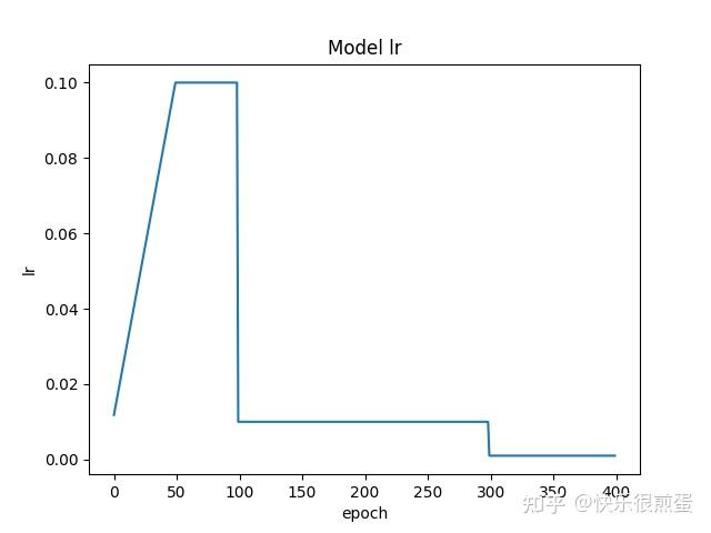
绘制学习率曲线,从start_epoch开始到epoch=400(不包含)截止,动态调整学习率策略选择的是“预热学习率”。
初始学习率为0.1(在optimizer内设置),epoch=50(warmup_iters)之前学习率以0.1斜率(warmup_factor)线性(warmup_method)上升到0.1(初始学习率),epoch=50(warmup_iters)到epoch=100(milestones)之间学习率都是0.1(初始学习率),epoch=100(milestones)和300时(milestones)分别降到前一个学习率的0.1倍(gamma)。
import math
import torch.optim as optim
import torch.nn as nn
from bisect import bisect_right


class WarmupLR(optim.lr_scheduler._LRScheduler):
    def __init__(self, optimizer, warmup_steps, last_epoch=-1):
        self.warmup_steps = warmup_steps
        super().__init__(optimizer, last_epoch)

    def get_lr(self):
        if self.last_epoch < self.warmup_steps:
            return [base_lr * (self.last_epoch + 1) / self.warmup_steps for base_lr in self.base_lrs]
        else:
            return [base_lr * math.exp(-(self.last_epoch - self.warmup_steps + 1) * self.gamma) for base_lr in
                    self.base_lrs]


class WarmupMultiStepLR(torch.optim.lr_scheduler._LRScheduler):
    def __init__(
        self,
        optimizer,
        milestones,
        gamma=0.1,
        warmup_factor=1/3,
        warmup_iters=100,
        warmup_method="linear",
        last_epoch=-1,
    ):
        if not list(milestones) == sorted(milestones):
            raise ValueError(
                "Milestones should be a list of" " increasing integers. Got {}",
                milestones,
            )

        if warmup_method not in ("constant", "linear"):
            raise ValueError(
                "Only 'constant' or 'linear' warmup_method accepted"
                "got {}".format(warmup_method)
            )
        self.milestones = milestones
        self.gamma = gamma
        self.warmup_factor = warmup_factor
        self.warmup_iters = warmup_iters
        self.warmup_method = warmup_method
        super(WarmupMultiStepLR, self).__init__(optimizer, last_epoch)

    def get_lr(self):
        warmup_factor = 1
        if self.last_epoch < self.warmup_iters:
            if self.warmup_method == "constant":
                warmup_factor = self.warmup_factor
            elif self.warmup_method == "linear":
                alpha = self.last_epoch / self.warmup_iters
                warmup_factor = self.warmup_factor * (1 - alpha) + alpha
        return [
            base_lr
            * warmup_factor
            * self.gamma ** bisect_right(self.milestones, self.last_epoch)
            for base_lr in self.base_lrs
        ]

if __name__ == "__main__":
    import matplotlib.pyplot as plt
    import numpy as np

    start_epoch = 0

    class Net(nn.Module):
        def __init__(self):
            super(Net, self).__init__()
            self.layer = nn.Linear(10, 2)
            self.layer2 = nn.Linear(2, 10)

        def forward(self, input):
            return self.layer(input)
    model = Net()  # 生成网络
    optimizer = optim.Adam(model.parameters(), lr=0.1)  # 生成优化器
    lr_scheduler = WarmupMultiStepLR(optimizer=optimizer,
                                         milestones=[100, 300],
                                         gamma=0.1,
                                         warmup_factor=0.1,
                                         warmup_iters=50,
                                         warmup_method="linear",
                                         last_epoch=-1)

    lr_list = []
    for epoch in range(start_epoch, 400):
        optimizer.step()
        lr_scheduler.step()
        lr_list.append(float(optimizer.state_dict()['param_groups'][0]['lr']))
        print('epoch', epoch, 'lr', float(optimizer.state_dict()['param_groups'][0]['lr']))

    plt.plot(np.arange(start_epoch, start_epoch + len(lr_list)), lr_list, label="train lr")
    plt.xlabel('epoch')
    plt.ylabel("lr")
    plt.title('Model lr')
    plt.show()
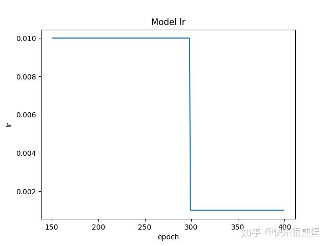
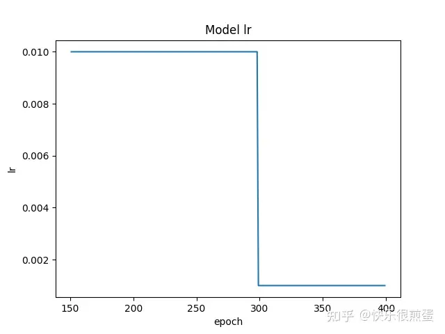
如果从epoch=151开始画:
start_epoch = 151
lr_list = []
for epoch in range(start_epoch, 400):
    optimizer.step()
    lr_scheduler.step()
    lr_list.append(float(optimizer.state_dict()['param_groups'][0]['lr']))
    print('epoch', epoch, 'lr', float(optimizer.state_dict()['param_groups'][0]['lr']))

plt.plot(np.arange(start_epoch, start_epoch + len(lr_list)), lr_list, label="train lr")
plt.xlabel('epoch')
plt.ylabel("lr")
plt.title('Model lr')
plt.show()
最后说一嘴,如果发现从断点继续训练之后损失函数和以往的数值相差特别大,那可能是几个load_state_dict()没做,以及epoch不对,还有就是model、optimizer、lr_scheduler的顺序。这里尤其需要注意lr_scheduler,按理说重新定义lr_scheduler,并让last_epoch=断点epoch也是可以继续训练的,但一定要看清lr_scheduler.step()放在了哪里,是不是在epoch下而不是batch下。
optimizer.step()
lr_scheduler.step()
lr_list.append(float(optimizer.state_dict()['param_groups'][0]['lr']))
 print('epoch', epoch, 'lr', float(optimizer.state_dict()['param_groups'][0]['lr']))

plt.plot(np.arange(start_epoch, start_epoch + len(lr_list)), lr_list, label="train lr")
plt.xlabel('epoch')
plt.ylabel("lr")
plt.title('Model lr')
plt.show()
最后说一嘴,如果发现从断点继续训练之后损失函数和以往的数值相差特别大,那可能是几个load_state_dict()没做,以及epoch不对,还有就是model、optimizer、lr_scheduler的顺序。这里尤其需要注意lr_scheduler,按理说重新定义lr_scheduler,并让last_epoch=断点epoch也是可以继续训练的,但一定要看清lr_scheduler.step()放在了哪里,是不是在epoch下而不是batch下。
推荐阅读:
各部分详情:(持续更新中…)
1. 机器学习
- 机器学习(一) 本文(3万字) | 机器学习概述 |-CSDN博客
- 机器学习(二) 本文(2.5万字) | KNN算法原理及Python复现 |-CSDN博客
- 机器学习(三) 本文(3万字) | 线性回归LR原理 | Python复现 |-CSDN博客
- 机器学习(四) 本文(2万字) | 梯度下降GD原理 | Python复现 |-CSDN博客
2. 深度学习与目标检测
3. YOLOv5
-
YOLOv5系列(一) 本文(1.2万字) | 项目结构 | 罗列全部函数与方法 | 全网最全代码调用关系图 |-CSDN博客
-
YOLOv5系列(二) 本文(1.1万字) | 解析配置文件yolov5s.yaml |_yolov5配置文件中-1可以用其它来代替吗-CSDN博客
-
YOLOv5系列(十二) 本文(1.5万字) | 解析数据增强部分augmentations | 逐行代码注释解析-CSDN博客
-
YOLOv5系列(十三) 本文(2万字) | 解析torch工具部分torch_utils | 逐行代码注释解析-CSDN博客
-
YOLOv5系列(十四) 本文(1.3万字) | 解析数据集处理部分dataloaders | 逐行代码注释解析-CSDN博客
-
YOLOv5系列(二十) 本文(4万字) | 训练自己的数据集 |利用labelimg标注数据集 | 划分自建数据集 | 从环境配置到数据及划分再到训练-CSDN博客
-
YOLOv5系列(二十三) 本文(2.5万字) | 自动混合精度AMP | 指数移动平均EMA | Test Time Augmentation(TTA) |-CSDN博客
-
YOLOv5系列(二十五) 本文(2万字) | 从二值损失基本原理到YOLOv5损失 | Binary Cross-Entropy | YOLOv5 LOSS |-CSDN博客
-
YOLOv5系列(二十七) 本文(2万字) | YOLOv5插值 | | Upsample | UpsamplingBilinear2D | UpsamplingNearest2D |-CSDN博客
-
YOLOv5系列(二十八) 本文(2万字) | 可视化工具 | Comet | ClearML | Wandb | Visdom |-CSDN博客
-
YOLOv5系列(二十九) 本文(1万字) | 多模型推理预测(Model Ensemble) | 参数重结构化(融合Conv+BatchNorm2d) |-CSDN博客
-
YOLOv5系列(三十一) 本文(1.5万字) | 标签平滑(Label Smoothing) | Focal Loss损失函数 | 学习率预热Warmup |-CSDN博客
-
YOLOv5系列(三十二) 本文(2.5万字) | 再次解读yaml文件 | 从yaml到模型结构的具体实施细节 | 魔改模型结构两头 | 四头 | 等 |-CSDN博客
4. YOLOv5改进
-
YOLOv5改进系列(四) 本文(2.5万字) | 更换Neck | BiFPN | AFPN | BiFusion |-CSDN博客
-
YOLOv5改进系列(六) 本文(5万字) | 更换损失函数 | GIoU | DIoU | CIoU | EIoU | AlphaIoU | SIoU | WIoU |-CSDN博客
-
YOLOv5改进系列(十四) 本文(1.2万字) | 更换减轻模型的复杂度同时提升精度GSConv+Slim-neck |-CSDN博客
-
YOLOv5改进系列(十六) 本文(1.2万字) |引入FasterNet | PConv |backbone |-CSDN博客
5. YOLOv8及其改进
6. Python与PyTorch
- Python与Pytorch系列(一) 本文(2万字) | 解析python中的pandas.read_csv() | pandas.read_json() | pandas.read_excel()-CSDN博客
- Python与Pytorch系列(二) 本文(1.8万字) | 解析Opencv, Matplotlib, PIL | 三者之间的转换 | 三者对JPG和PNG读取和写入 |-CSDN博客
- Python与PyTorch系列(三) 本文(4.2万字) | 解读Python中的装饰器 | 复现各种装饰器 | 给出众多实用装饰器 |-CSDN博客
- Python与PyTorch系列(四) 本文(1万字) | 解析python中的魔术方法 |-CSDN博客
- Python与PyTorch系列(五) 本文(5万字) | 解析PyTorch中Hook函数 |-CSDN博客
7. 工具
- Python与PyTorch系列(三) 本文(4.2万字) | 解读Python中的装饰器 | 复现各种装饰器 | 给出众多实用装饰器 |-CSDN博客
- 工具系列(二) 本文(3万字) | 解读在Windows下配置GPU环境(以YOLOv5为例) | 并使用Pytorch训练一个简单的图像分类模型(GPU) |-CSDN博客
- 工具系列(三) 本文(1.5万字) | 解析glob.glob | os.walk |-CSDN博客
- 工具系列(四) 本文(5万字) | pytorch中使用tensorboard进行可视化 | 可视化 | tensorboard |-CSDN博客
8. 小知识点
-
小知识点系列(一) 本文(2.2万字) | 图像变换 | 平移缩放旋转翻错切 | 仿射变换与透视变换 | 代码复现 |-CSDN博客
-
小知识点系列(四) 本文(1万字) | 解析Bounding Box Regression | 边界框回归 |-CSDN博客
-
小知识点系列(五) 本文(5万字) | 解读深度学习中的八种卷积 | pytorch中Conv1d、Conv2d,Conv3d | 空洞卷积 | 转置卷积 | 深度可分离卷积 |-CSDN博客
-
小知识点系列(六) 本文(1.5万字) | 理解深度学习中计算量(FLOPs)和参数量(Params) | 四种计算方法总结 |-CSDN博客