[PyTorch] nn.Conv2d与F.cond2d的手写实现（nn、nn.functional、Conv、Conv2d、卷积、实现、卷积核个数、stride、im2col、输出通道数、特征图）

0. 学习路线

本文讲解普通卷积。

1. PyTorch 中卷积的分类

在 PyTorch 中，普通卷积一般有三种：

1. nn.conv1d()：用于一维信号（例如时间序列数据）的卷积层。
2. nn.conv2d()：用于二维图像的卷积层，常用于处理图像数据。
3. nn.conv3d()：用于三维数据（例如视频数据或三维扫描数据）的卷积层。

这里我们主要讲解 nn.conv2d，因为 nn.conv1d 和 nn.conv3d 可以当做 nn.conv2d 那样去计算。

2. nn.Conv2d 和 nn.conv2d 的区别

我们在搜索 conv2d 时会发现有两种：

1. Conv2d
2. conv2d

二者的字母 C 一个是大写的一个是小写的，那么二者有区别吗？答案是肯定的，具体区别如下：

• Conv2d：是用于构造卷积层的类（Class），用于创建卷积层对象。
• conv2d：是一个函数（function），用于执行卷积操作，它直接进行卷积计算。

注意❗️：二者除了本质上有区别外，还存在一些值得我们关注的差异：

1. Conv2d 是用于构造卷积层的类（Class），用于创建卷积层对象。这是一个模型组件，它具有可学习的参数（如权重和偏置），并且在模型训练过程中会通过反向传播更新这些参数。
2. conv2d：因为这个卷积是一个函数（function），用于执行卷积操作，它直接进行卷积计算。这个函数没有可学习的参数，因此在模型训练过程中不能通过反向传播来调整它的参数。

由于 Conv2d 是一个卷积层的类，而且可以自动管理权重和偏置的学习过程，通常情况下，我们在构建深度学习模型时会使用 nn.Conv2d 而不是 nn.conv2d。在定义模型结构时，Conv2d 通常作为卷积层的组件使用，而在模型的前向传播过程中，我们会使用 conv2d 函数来执行具体的卷积操作。这样，Conv2d 和 conv2d 可以协同工作，形成完整的深度学习模型。

3. torch.nn.Conv2d

CLASStorch.nn.Conv2d(in_channels, out_channels, kernel_size, stride=1, padding=0, 
					 dilation=1, groups=1, bias=True, padding_mode='zeros', 
					 device=None, dtype=None)

以上是 PyTorch 中 torch.nn.Conv2d 类的构造函数（ __init__ 方法），目的用于创建一个二维卷积层。

PyTorch 官方 API 地址：https://pytorch.org/docs/1.12/generated/torch.nn.Conv2d.html?highlight=conv2d#torch.nn.Conv2d

参数说明如下：

1. in_channels（int）：输入图像的通道数。对于彩色图像，通常为 3（RGB），对于灰度图像，通常为 1。

2. out_channels（int）：输出通道数，也就是卷积核的数量，每个卷积核会生成一个输出通道。也就是卷积操作后生成的特征图数量。

3. kernel_size（int 或 tuple）：卷积核的大小。如果是 int 类型，表示卷积核的高度和宽度相等；如果是 tuple 类型，如 kernel_size=(3, 5)，表示卷积核的高度和宽度分别为 3 和 5。

4. stride（int 或 tuple，可选）：卷积操作的步长（stride）。如果是 int 类型，表示在高度和宽度方向上的步长相等；如果是 tuple 类型，如 stride=(2, 1)，表示在高度和宽度方向上的步长分别为 2 和1。默认值为 1。

5. padding（int 或 tuple，可选）：在 输入图像的周围 添加零值填充（padding）的层数。如果是 int 类型，表示在高度和宽度方向上的填充层数相等；如果是 tuple 类型，如 (1, 2)，表示在高度和宽度方向上的填充层数分别为 1 和 2。默认值为 0。 —— 使用什么填充需要看 padding_mode

6. dilation（int 或 tuple，可选）：控制卷积核内部元素之间的间距（dilation）。如果是 int 类型，表示在卷积核内部元素之间的间距在高度和宽度方向上相等；如果是 tuple 类型，如 (2, 2)，表示在高度和宽度方向上的间距分别为 2。默认值为 1（不使用膨胀卷积）。

7. groups（int，可选）：控制输入和输出通道之间的连接方式。当 groups>1 时，表示使用分组卷积，将输入通道和输出通道分成 groups 组，并分别进行卷积操作。默认值为 1，即普通卷积。

8. bias（bool，可选）：是否添加偏置项。如果为 True，表示会为每个输出通道添加 一个 偏置项；如果为 False，表示不添加偏置项。默认值为 True。

9. padding_mode（str，可选）：选择 padding 的模式。可选值为 ‘zeros’（默认值）或 ‘reflect’。

   • ‘zeros’ 表示使用 0 进行填充
   • ‘reflect’ 表示使用输入图像的边界值进行填充

10. device（torch.device，可选）：指定该层运行在哪个设备上（例如 CPU 或 GPU）。默认值为 None，表示使用默认设备。

11. dtype（torch.dtype，可选）：指定该层的数据类型。默认值为 None，表示使用默认数据类型。

3.1 卷积过程示意图

输入特征图大小为 4×4；kernel_size=3, stride=1, padding=0, bias=False

以上其实是 nn.conv1d 的卷积过程，nn.conv2d 本质上是一样的。

值得注意的是❗️：

1. 在卷积操作中，卷积核的滑动方式是走 回字形轨迹 而不是 Z 型轨迹（这里的 gif 动图是有问题的，它走的是 Z 型轨迹）。

确切来说是一个 “弓” 字型轨迹。

2. 上面是没有偏置的，如果有偏置，也不影响图片，只不过输出特征图会沿着通道方向加上一个偏置（输出特征图一共会加 out_channels 个偏置）。

偏置项的作用是为了引入对输入数据的线性偏移，使模型能够更好地拟合数据。在卷积层中，对于每个输出通道，都有一个对应的偏置项。在进行卷积操作时，每个输出通道的卷积结果会与相应的偏置项 相加，从而得到输出特征图。

在模型训练过程中，nn.Conv2d 会不断通过反向传播更新自己的参数，即 ①卷积核参数和 ②偏置项：

1. 卷积核参数（Weights）：每个卷积核都是一个可学习的参数矩阵，用于在输入图像上执行特征提取。nn.Conv2d 层会学习这些卷积核的参数，使得它们能够有效地捕捉输入图像中的不同特征。

2. 偏置项（Bias）：如果在 nn.Conv2d 中使用了偏置（bias=True），那么每个输出通道都会有一个可学习的偏置项。这些偏置项用于引入对输入数据的线性偏移，使得模型能够更好地拟合数据。

❗️❗️我们一定不要搞错，特征图参数不是我们所考虑的内容，更新参数一定是更新卷积的参数，即卷积核参数和偏置项。

3.2 卷积代码示例

import torch
import torch.nn as nn
import torch.nn.functional as F


# 实例化一个二维卷积
conv_layer = torch.nn.Conv2d(in_channels=1, out_channels=1, kernel_size=(3, 3), 
                             stride=1, padding=0, bias=False)

# 定义一个输入特征图
input_feature_map = torch.randn(size=[1, 1, 4, 4])  # BS, C, H, W

# 将输入特征图送入卷积得到输出特征图
output_feature_map = conv_layer(input_feature_map)


print(f"----------------输入特征图--------------------")
print(f"input feature map: {
      
      input_feature_map}")
print(f"input feature map.shape: {
      
      input_feature_map.shape}")
"""
input feature map: tensor([[[[ 1.3073, -1.5880, -0.9452,  0.4990],
          [ 0.4691, -0.0185,  1.7039,  0.4509],
          [ 1.0158,  1.7649, -1.1296,  0.0249],
          [ 1.7177, -1.5447,  0.0709,  1.0709]]]])
input feature map.shape: torch.Size([1, 1, 4, 4])
"""

print(f"\r\n----------------输出特征图--------------------")
print(f"output feature map: {
      
      output_feature_map}")
print(f"output feature map.shape: {
      
      output_feature_map.shape}")
print(f"output feature map.shape: {
      
      output_feature_map.shape}")
print(f"output feature map.dtype: {
      
      output_feature_map.dtype}")
print(f"output feature map.device: {
      
      output_feature_map.device}")
print(f"output feature map.size(): {
      
      output_feature_map.size()}")
print(f"output feature map.dim(): {
      
      output_feature_map.dim()}")
print(f"output feature map.ndim: {
      
      output_feature_map.ndim}")
print(f"output feature map.numel(): {
      
      output_feature_map.numel()}")
"""
output feature map: tensor([[[[ 1.5613, -0.6933],
          [-1.4673, -0.6003]]]], grad_fn=<ConvolutionBackward0>)
output feature map.shape: torch.Size([1, 1, 2, 2])
output feature map.shape: torch.Size([1, 1, 2, 2])
output feature map.dtype: torch.float32
output feature map.device: cpu
output feature map.size(): torch.Size([1, 1, 2, 2])
output feature map.dim(): 4
output feature map.ndim: 4
output feature map.numel(): 4
"""

print(f"\r\n----------------卷积层--------------------")
print(f"conv_layer.in_channels: {
      
      conv_layer.in_channels}")
print(f"conv_layer.out_channels: {
      
      conv_layer.out_channels}")
print(f"conv_layer.kernel_size: {
      
      conv_layer.kernel_size}")
print(f"conv_layer.stride: {
      
      conv_layer.stride}")
print(f"conv_layer.padding: {
      
      conv_layer.padding}")
print(f"conv_layer.bias: {
      
      conv_layer.bias}")
print(f"conv_layer.weight: {
      
      conv_layer.weight}")
print(f"conv_layer.weight.shape: {
      
      conv_layer.weight.shape}")
"""
conv_layer.in_channels: 1
conv_layer.out_channels: 1
conv_layer.kernel_size: (3, 3)
conv_layer.stride: (1, 1)
conv_layer.padding: (0, 0)
conv_layer.bias: None
conv_layer.weight: Parameter containing:
tensor([[[[ 0.1567, -0.0156, -0.1600],
          [-0.2636, -0.2253,  0.2938],
          [ 0.1223,  0.3061, -0.1196]]]], requires_grad=True)
conv_layer.weight.shape: torch.Size([1, 1, 3, 3])
"""

3.3 特征图（Feature map）可查看的属性

在PyTorch中，一个特征图（Feature Map）是一个由 torch.Tensor 表示的多维数组。我们可以使用 torch.Tensor 的属性和方法来查看特征图的相关信息。

一般来说，以下是我们可以查看的特征图的一些属性：

1. shape：使用 .shape 属性可以查看特征图的形状，它告诉你特征图的维度大小，如 (batch_size, channels, height, width)。

2. dtype：使用 .dtype 属性可以查看特征图的数据类型，通常是 float32 或 float64。

3. device：使用 .device 属性可以查看特征图所在的设备，如 CPU 或 GPU。

4. size()：使用 .size() 方法可以查看特征图的尺寸，它返回一个元组 tuple，包含特征图在每个维度上的大小。

5. dim()：使用 .dim() 方法可以查看特征图的维度数量。

6. ndim：使用 .ndim 属性可以查看特征图的维度数量，与 dim() 方法功能相同。

7. numel()：使用 .numel() 方法可以查看特征图的元素总数，即特征图中所有元素的个数。

除了这些基本属性，我们还可以通过 索引 和 切片 的操作查看特征图中的具体数值。例如，使用 tensor[0] 可以查看第一个样本（batch_size 维度）的特征图，tensor[:, 0] 可以查看第一个通道的特征图，tensor[:, :, 2:5, 3:6] 可以查看特定高度和宽度范围的子集。

在实际使用中，特征图的属性可以帮助我们了解数据的形状和类型，有助于调试和确认模型的输出。

重点记忆：.shape、.device 即可。

3.4 卷积层（Convolution）可查看的属性

对于定义的 nn.Conv2d，我们可以查看以下属性：

1. in_channels：输入通道数。

2. out_channels：输出通道数。

3. kernel_size：卷积核的大小。

4. stride：卷积操作的步长。

5. padding：填充层数。

6. dilation：卷积核元素之间的间距。

7. groups：输入和输出通道之间的连接方式。

8. bias：是否有偏置项。

9. padding_mode：填充的模式。

10. weight：卷积核的权重参数。

11. bias：偏置项的参数。

这些属性描述了卷积层的配置和参数信息，它们可以帮助我们了解和确认卷积层的设置。要查看这些属性的值，我们可以直接通过 nn.Conv2d 对象来访问它们，例如：

print(nn.conv2d.in_channels)  # 输出输入通道数
print(nn.conv2d.out_channels)  # 输出输出通道数
print(nn.conv2d.kernel_size)  # 输出卷积核的大小
print(nn.conv2d.stride)  # 输出卷积操作的步长
print(nn.conv2d.padding)  # 输出填充层数
print(nn.conv2d.dilation)  # 输出卷积核元素之间的间距
print(nn.conv2d.groups)  # 输出输入和输出通道之间的连接方式
print(nn.conv2d.bias)  # 输出是否有偏置项
print(nn.conv2d.padding_mode)  # 输出填充的模式
print(nn.conv2d.weight)  # 输出卷积核的权重参数
print(nn.conv2d.bias)  # 输出偏置项的参数

这些属性信息是创建 nn.Conv2d 对象时指定的参数，也包含了该卷积层的权重参数和偏置项参数。

4. torch.nn.functional.conv2d

PyTorch 官方 API 地址：https://pytorch.org/docs/1.12/generated/torch.nn.functional.conv2d.html?highlight=conv2d#torch.nn.functional.conv2d

torch.nn.functional.conv2d(input, weight, bias=None, stride=1, 
						   padding=0, dilation=1, groups=1) -> Tensor

torch.nn.functional.conv2d 是 PyTorch 中用于执行二维卷积操作的函数。它和 torch.nn.Conv2d 是两种不同的实现方式，其中 torch.nn.functional.conv2d 是一个函数，而 torch.nn.Conv2d 是一个类。 torch.nn.functional.conv2d 函数提供了更灵活的操作，可以在函数调用时直接指定卷积核的权重参数，而不需要像类那样在初始化时定义。

参数说明：

• input：输入的特征图，一个四维张量，形状为 (batch_size, in_channels, height, width)。

• weight：卷积核的权重参数，一个四维张量，形状为 (out_channels, in_channels, kernel_height, kernel_width)。

• bias：可选的偏置项参数，一个一维张量，形状为 (out_channels,)。默认值为 None，表示不使用偏置项。

• stride：卷积操作的步长，可以是一个整数或一个元组 (stride_height, stride_width)。默认值为 1。

• padding：填充层数，可以是一个整数或一个元组 (padding_height, padding_width)。默认值为 0。

• dilation：卷积核元素之间的间距，可以是一个整数或一个元组 (dilation_height, dilation_width)。默认值为 1。

• groups：输入和输出通道之间的连接方式，控制卷积操作的分组，可以是一个整数。默认值为 1，表示普通卷积。

该函数的返回值是执行卷积操作后得到的特征图，一个四维张量，形状为 (batch_size, out_channels, output_height, output_width)。

使用torch.nn.functional.conv2d函数时，需要手动传入卷积核的权重参数。它通常在自定义模型或一些特定的卷积操作中使用，而在大多数情况下，建议使用torch.nn.Conv2d类，它更简单方便，自动管理卷积核的权重参数。

4.1 卷积过程示意图

与 torch.nn.Conv2d 没有区别。

4.2 卷积代码示例

import torch
import torch.nn as nn
import torch.nn.functional as F


# 固定随机数种子
torch.manual_seed(10010)

# 定义一个输入特征图
input_feature_map = torch.randn(size=[1, 1, 4, 4])  # BS, C, H, W

# 实例化一个二维卷积
conv_layer = torch.nn.Conv2d(in_channels=1, out_channels=1, kernel_size=(3, 3),
                             stride=1, padding=0, bias=False)

# 定义卷积核参数
kernel_weight = torch.Tensor([[[[-0.0765,  0.1716,  0.2779],
                                [-0.1685, -0.1217,  0.0160],
                                [0.1584, -0.2000, -0.2148]]]])

# 将输入特征图送入卷积得到输出特征图
output_feature_map_1 = conv_layer(input_feature_map)

# 直接使用卷积得到输出特征图
output_feature_map_2 = torch.nn.functional.conv2d(
    input=input_feature_map, weight=kernel_weight, bias=None, stride=1, padding=0)  # F.conv2d()也可以

print(f"\r\n----------------输出特征图--------------------")
print(f"output feature map 1: {
      
      output_feature_map_1}")
print(f"output feature map 2: {
      
      output_feature_map_2}")

结果：

output feature map 1: tensor([[[[ 1.3038,  0.0875],
          [-0.8772, -0.1317]]]], grad_fn=<ConvolutionBackward0>)
output feature map 2: tensor([[[[ 1.3037,  0.0875],
          [-0.8773, -0.1318]]]])

grad_fn=<ConvolutionBackward0> 是输出特征图在计算时生成的一个梯度函数（gradient function），它用于跟踪计算图，并在反向传播时计算梯度。这是因为 output_feature_map_1 是通过调用 conv_layer(input_feature_map) 来计算的，它是一个由 torch.nn.Conv2d 类型的对象进行操作的结果。由于 torch.nn.Conv2d 类自带梯度计算功能，因此在计算 output_feature_map_1 时，PyTorch自动在其上创建了梯度函数。

而对于 output_feature_map_2，它是通过调用 torch.nn.functional.conv2d 函数计算得到的。这是一个纯函数（pure function），它没有任何与梯度相关的操作，因此在计算 output_feature_map_2 时，并不会生成梯度函数。

当我们调用类方法或属性时，PyTorch会在这些操作上自动创建梯度函数。但是对于纯函数，由于它们不涉及可训练参数的梯度计算，所以不会生成梯度函数。

5. 卷积运算示意

卷积和池化后形状计算公式分别如下：

没有空洞卷积的计算：
$${H/W}_i^{conv/pool}=\frac{{H/W}_i^{\mathrm{in}}+2p_i-k_i}{s_i}+1$$

带有空洞卷积后的计算：

$${H/W}_i^{\mathrm{dialated}\mathrm{conv}}=\frac{{H/W}_i^{\mathrm{in}}+2p_i-d_i\times (k_i-1)}{s_i}+1$$

卷积: 向下取整
池化: 向上取整

5.1 stride=1, padding=0

根据上面的公式可知，输出特征图大小为：

$$\begin{array}{rl}{H/W}_i& =\frac{{H/W}_i^{\mathrm{in}}+2p_i-k_i}{s_i}+1\\ & =\frac{5+2\times 0-3}{1}+1\\ & =3\end{array}$$

即输出特征图的宽度和高度为 $3\times 3$。

❗️注意❗️：特征图和卷积核的乘法是点乘（element-wise multiplication），也被成为逐元素乘法或内积，即对应位置元素相乘最后再求和，而非我们理解的矩阵乘法。

5.2 stride=2, padding=1

根据上面的公式可知，输出特征图大小为：

$$\begin{array}{rl}{H/W}_i& =\frac{{H/W}_i^{\mathrm{in}}+2p_i-k_i}{s_i}+1\\ & =\frac{5+2\times 1-3}{2}+1\\ & =3\end{array}$$

即输出特征图的宽度和高度为 $3\times 3$。我们发现，stride=1, padding=0 和 stride=2, padding=1 输出特征图的 宽度和高度 是一样的。

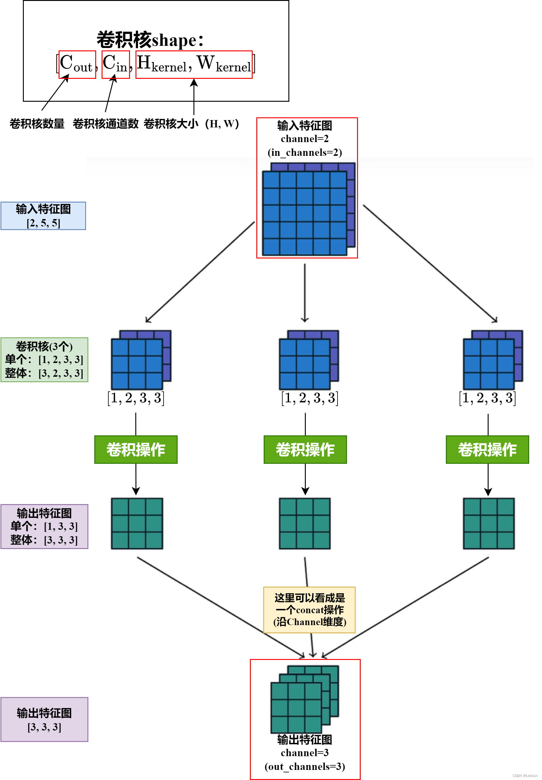
5.3 in_channels=2, out_channels=3, kernel_size=3, stride=1, padding=0

5.1 和 5.2 中都是单通道特征图在卷积中的运算，但在实际任务中，我们的输入图像一般是多通道的，特征图也是多通道的，因此我们看一下下面的这种情况。

5.4 ❗️卷积核注意事项❗️

5.4.1 输出特征图通道数（输出特征图数量）

输出特征图的通道数是由卷积核的个数决定的，因为一个卷积核生成一张特征图。即 out_channels 就是输出特征图的通道数。

5.4.2 卷积核个数（数量）

对于一个卷积层而言，卷积核的数量等于 out_channels，而不是 in_channels * out_channels。

在卷积层中，每个输出通道都有一个对应的卷积核。卷积核的形状是 (out_channels, in_channels, kernel_height, kernel_width)，其中 out_channels 是输出通道的数量，而 in_channels 是输入通道的数量。这意味着每个输出通道都需要一个大小为 (in_channels, kernel_height, kernel_width) 的卷积核与输入通道进行卷积运算。

因此，卷积核的数量就是输出通道的数量 out_channels，而不是 in_channels * out_channels。每个输出通道对应一个卷积核，卷积核的数量等于输出通道的数量。

❗️注意❗️：卷积过程中卷积核的数量（即 out_channels）在 __init__ 方法中就已经确定好了，所以说这个卷积层的输出通道数就已经确定了。我们在模型训练过程中一般是不会突然改变某个 nn.Conv2d 层的 out_channels 参数 —— 其他参数也是同理（要记住 nn.Conv2d 是一个类而非一个函数）。

• 一旦实例化了 nn.Conv2d 对象，并在 __init__ 方法中指定了参数，这些参数就会在整个卷积层的生命周期中保持不变。
• 模型的结构在训练过程中保持不变，参数的更新只发生在权重和偏置等可以学习的参数上，而不是在 nn.Conv2d 层的配置参数上

5.5 设置 padding 使得 输入输出特征图尺寸不变

方法1：

padding = (kernel_size - 1) // 2  # kernel_size 必须为奇数

方法2：

padding = (kernel_size * 2 + 1) // 2  # kernel_size 可以为偶数

6. 滑动相乘实现 F.conv2d()

接下来我们将会按照这样的运算流程进行卷积的代码实现。

6.1 F.conv2d() 的代码实现（忽略 batch size 和 channel）

import torch
import torch.nn as nn
import torch.nn.functional as F
import math


def matrix_multiplication_for_conv2d(input, kernel, stride=1, padding=0, bias=None):
    """使用原始的矩阵运算实现二维卷积(先不考虑batch_size和channel维度)

    Args:
        input (Tensor): 输入特征图，形状为 [H, W]
        kernel (Tensor): 卷积核，形状为 [kernel_h, kernel_w]
        stride (int, optional): 步长. Defaults to 1.
        padding (int, optional): 填充. Defaults to 0.
        bias (Tensor, optional): 偏置. Defaults to None.

    Returns:
        _type_: 输出特征图
    """
    # 是否需要进行padding
    if padding > 0:
        input = F.pad(input, (padding, padding, padding, padding))  # 上下左右都需要pad
    
    # 获取输入大小
    input_h, input_w = input.shape
    kernel_h, kernel_w = kernel.shape
    
    # 计算输出特征图尺寸（卷积尺寸向下取整）Note：先进行padding，所以在计算输出特征图尺寸时不用考虑padding的值了！
    output_w  = math.floor((input_w - kernel_w) / stride) + 1
    output_h  = math.floor((input_h - kernel_h) / stride) + 1
    
    # 随机初始化一个要输出的矩阵
    output = torch.zeros([output_h, output_w])
    
    # 进行两层的遍历（先H再W）
    for h in range(0, input_h - kernel_h + 1, stride):  # 对高度进行遍历（步长为stride）
        for w in range(0, input_w - kernel_w + 1, stride):  # 对宽度进行遍历（步长为stride）
            # 进行矩阵的逐元素相乘
            region = input[h: h + kernel_h, w: w + kernel_w]  # 取出要与卷积核进行点积的区域
            output[int(h / stride), int(w / stride)] = torch.sum(region * kernel)  # 进行点乘并赋值给输出的位置
            
    # 偏置(应该先完成所有的卷积运算，然后再添加偏置值)
    if bias is not None:
        output = output + bias
                
    return output


if __name__ == "__main__":
    # 固定随机数种子
    torch.manual_seed(10010)
    
    # 输入特征图
    input = torch.randn(size=[5, 5])  # BS, C, H, W
    
    kernel = torch.randn([3, 3])# 卷积核参数
    bias = torch.randn([1, ])  # 卷积核偏置 —— bias只与输出通道数有关（即卷积核个数）
    
    # PyTorch的结果
    res_pytorch = torch.nn.functional.conv2d(input=input.reshape(1, 1, input.shape[0], input.shape[1]), 
                                             weight=kernel.reshape(1, 1, kernel.shape[0], kernel.shape[1]), 
                                             stride=1, 
                                             padding=1, 
                                             bias=bias)
    print(f"PyTorch的结果:\r\n{
      
      res_pytorch.squeeze()}")

    #自己实现的结果
    res = matrix_multiplication_for_conv2d(input=input, 
                                           kernel=kernel, 
                                           stride=1, 
                                           padding=1, 
                                           bias=bias)
    print(f"自己实现的结果:\r\n{
      
      res}")

    # 对比两个Tensor对应位置的浮点数是否接近
    print(torch.allclose(res_pytorch, res))  # True    

结果如下：

PyTorch的结果:
tensor([[-0.8682,  0.0836,  2.4579,  7.9269, -0.2708],
        [-3.4977, -1.1559,  4.6909, -0.1927,  0.3715],
        [-1.3349, -0.7388, -8.6954, -1.6454,  0.0757],
        [-7.0991, -0.4209,  1.2751,  2.7073, -2.9031],
        [ 0.1042, -0.1368,  2.0605, -1.1924,  0.0251]])

自己实现的结果:
tensor([[-0.8682,  0.0836,  2.4579,  7.9269, -0.2708],
        [-3.4977, -1.1559,  4.6909, -0.1927,  0.3715],
        [-1.3349, -0.7388, -8.6954, -1.6454,  0.0757],
        [-7.0991, -0.4209,  1.2751,  2.7073, -2.9031],
        [ 0.1042, -0.1368,  2.0605, -1.1924,  0.0251]])

6.2 F.conv2d() 的代码实现（实现 batch size 和 channel）

6.2.1 方法 1

import torch
import torch.nn as nn
import torch.nn.functional as F
import math


def matrix_multiplication_for_conv2d_completed(input, kernel, stride=1, padding=0, bias=None):
    """使用原始的矩阵运算实现二维卷积(支持多通道和batch维度)

    Args:
        input (Tensor): 输入特征图，形状为 [Batchsize, C, H, W]
        kernel (Tensor): 卷积核，形状为 [out_channels, in_channels, kernel_h, kernel_w]
        stride (int, optional): 步长. Defaults to 1.
        padding (int, optional): 填充. Defaults to 0.
        bias (Tensor, optional): 偏置. Defaults to None.

    Returns:
        Tensor: 输出特征图
    """
    # 是否需要进行padding
    if padding > 0:
        input = F.pad(input, (padding, padding, padding, padding))  # 上下左右都需要pad
    
    # 获取输入大小
    batch_size, in_channels, input_h, input_w = input.shape
    out_channels, _, kernel_h, kernel_w = kernel.shape  # 第二个参数和 in_channels 是一样的
    
    # 计算输出特征图尺寸（卷积尺寸向下取整）Note：先进行padding，所以在计算输出特征图尺寸时不用考虑padding的值了！
    output_w  = math.floor((input_w - kernel_w) / stride) + 1
    output_h  = math.floor((input_h - kernel_h) / stride) + 1
    
    # 随机初始化一个要输出的矩阵
    output = torch.zeros([batch_size, out_channels, output_h, output_w])
    
    # 进行两层的遍历（先H再W）
    for h in range(0, input_h - kernel_h + 1, stride):  # 对高度进行遍历（步长为stride）
        for w in range(0, input_w - kernel_w + 1, stride):  # 对宽度进行遍历（步长为stride）
            # 进行矩阵的逐元素相乘
            region = input[:, :, h: h + kernel_h, w: w + kernel_w]  # 取出要与卷积核进行点积的区域
            output[:, :, int(h / stride), int(w / stride)] = torch.sum(region * kernel, dim=(1, 2, 3))  # 进行点乘并赋值给输出的位置
            
    # 偏置(应该先完成所有的卷积运算，然后再添加偏置值)
    if bias is not None:
        output = output + bias.view(1, -1, 1, 1)
                
    return output


if __name__ == "__main__":
    # 固定随机数种子
    torch.manual_seed(10010)
    
    # 输入特征图
    input = torch.randn(size=[2, 3, 5, 5])  # Batchsize, C, H, W
    
    kernel = torch.randn([2, 3, 3, 3])  # 卷积核参数，形状为 [out_channels, in_channels, kernel_h, kernel_w]
    bias = torch.randn([2, ])  # 卷积核偏置 —— bias只与输出通道数有关（即卷积核个数）
    
    # PyTorch的结果
    res_pytorch = F.conv2d(input=input, weight=kernel, stride=1, padding=1, bias=bias)
    print(f"PyTorch的结果:\r\n{
      
      res_pytorch.squeeze()}")

    #自己实现的结果
    res = matrix_multiplication_for_conv2d_completed(input=input, kernel=kernel, stride=1, padding=1, bias=bias)
    print(f"自己实现的结果:\r\n{
      
      res}")

    # 对比两个Tensor对应位置的浮点数是否接近
    print(torch.allclose(res_pytorch, res))  # True

结果如下：

PyTorch的结果:
tensor([[[[  3.0275,   4.8720,  -3.9974,   5.1608,   0.9514],
          [ 12.4525,   7.4182,   4.6702,   9.7314,  -4.3571],
          [ -3.2892,   3.6016,  10.4584,   3.5384,   0.3544],
          [  8.7312,   2.6497,   9.4672,   1.7016,   2.4650],
          [  7.2345,   2.1328,   7.7006,   0.4131,  13.1020]],

         [[  5.9256,  -5.6192,  -4.8512,  -3.4734,   1.9928],
          [  4.2990,  -1.4098,   3.8647,  -6.9448,  -1.0597],
          [ -6.0460,   8.2837,  -4.8912,   0.2388,  -4.4331],
          [  0.4701,   0.0266,  -8.2944,  -2.9790, -10.2942],
          [ -3.5228,  -0.0789,   2.3564,   0.3716,  -0.5882]]],


        [[[ -0.1347,   1.7058,   4.0682,   7.5516,   4.9627],
          [ -2.8487,   4.7063,   7.4273,  -4.6978,   4.9483],
          [  4.7545,   9.5539,  -2.7510,  15.1170,   5.1214],
          [  6.2537,   0.9930,  10.9024,  14.6522,  -6.8478],
          [ -0.6205,   1.6231,   5.5700,   9.6074,   3.6440]],

         [[ -0.5853,   7.7044,  -1.2999,   1.1914,  -4.6534],
          [ -4.9776,  -0.9076,   2.6359, -11.0334,   3.5623],
          [ -3.4314,   2.2645,  -4.6050,   0.9916,  -3.6573],
          [  0.5469,  -0.7690,   5.5431, -15.3839,  -4.1287],
          [ -5.7980,  -0.1221,  -6.2585,   0.1956,  -0.7817]]]])

自己实现的结果:
tensor([[[[  3.0275,   4.8720,  -3.9974,   5.1608,   0.9514],
          [ 12.4525,   7.4182,   4.6702,   9.7314,  -4.3571],
          [ -3.2892,   3.6016,  10.4584,   3.5384,   0.3544],
          [  8.7312,   2.6497,   9.4672,   1.7016,   2.4650],
          [  7.2345,   2.1328,   7.7006,   0.4131,  13.1020]],

         [[ -0.5853,   7.7044,  -1.2999,   1.1914,  -4.6534],
          [ -4.9776,  -0.9076,   2.6359, -11.0334,   3.5623],
          [ -3.4314,   2.2645,  -4.6050,   0.9916,  -3.6573],
          [  0.5469,  -0.7690,   5.5431, -15.3839,  -4.1287],
          [ -5.7980,  -0.1221,  -6.2585,   0.1956,  -0.7817]]],


        [[[  3.0275,   4.8720,  -3.9974,   5.1608,   0.9514],
          [ 12.4525,   7.4182,   4.6702,   9.7314,  -4.3571],
          [ -3.2892,   3.6016,  10.4584,   3.5384,   0.3544],
          [  8.7312,   2.6497,   9.4672,   1.7016,   2.4650],
          [  7.2345,   2.1328,   7.7006,   0.4131,  13.1020]],

         [[ -0.5853,   7.7044,  -1.2999,   1.1914,  -4.6534],
          [ -4.9776,  -0.9076,   2.6359, -11.0334,   3.5623],
          [ -3.4314,   2.2645,  -4.6050,   0.9916,  -3.6573],
          [  0.5469,  -0.7690,   5.5431, -15.3839,  -4.1287],
          [ -5.7980,  -0.1221,  -6.2585,   0.1956,  -0.7817]]]])

---

6.2.2 方法 2

import torch
import torch.nn as nn
import torch.nn.functional as F
import math


def matrix_multiplication_for_conv2d_full(input, kernel, stride=1, padding=0, bias=None):
    """使用原始的矩阵运算实现二维卷积(支持多通道和batch维度)

    Args:
        input (Tensor): 输入特征图，形状为 [Batchsize, C, H, W]
        kernel (Tensor): 卷积核，形状为 [out_channels, in_channels, kernel_h, kernel_w]
        stride (int, optional): 步长. Defaults to 1.
        padding (int, optional): 填充. Defaults to 0.
        bias (Tensor, optional): 偏置. Defaults to None.

    Returns:
        Tensor: 输出特征图
    """
    # 是否需要进行padding
    if padding > 0:
        # 上下左右都需要pad
        input = F.pad(input, (padding, padding, padding, padding, 0, 0, 0, 0))

    # 获取输入大小
    batch_size, in_channels, input_h, input_w = input.shape
    out_channels, in_channels, kernel_h, kernel_w = kernel.shape

    # 计算输出特征图尺寸（卷积尺寸向下取整）Note：先进行padding，所以在计算输出特征图尺寸时不用考虑padding的值了！
    output_w = math.floor((input_w - kernel_w) / stride) + 1
    output_h = math.floor((input_h - kernel_h) / stride) + 1

    # 随机初始化一个要输出的矩阵
    output = torch.zeros([batch_size, out_channels, output_h, output_w])  # BS, C, H, W

    for bs in range(batch_size):  # 样本层
        for out_c in range(out_channels):  # 输出通道层
            for in_c in range(in_channels):  # 输入通道层
                for h in range(0, input_h - kernel_h + 1, stride):  # 高度层
                    for w in range(0, input_w - kernel_w + 1, stride):  # 宽度层
                        # 进行矩阵的逐元素相乘
                        region = input[bs, in_c, h: h + kernel_h, w: w + kernel_w]  # 取出要与卷积核进行点积的区域
                        output[bs, out_c, int(h / stride), int(w / stride)] += torch.sum(region * kernel[out_c, in_c])

            # 偏置(应该先完成所有的卷积运算，然后再添加偏置值)
            if bias is not None:
                output[bs, out_c] += bias[out_c]

    return output


if __name__ == "__main__":
    # 固定随机数种子
    torch.manual_seed(10010)

    # 输入特征图
    input = torch.randn(size=[2, 2, 5, 5])  # BS, C, H, W

    kernel = torch.randn([3, input.shape[1], 3, 3])  # out_channels, in_channels, kernel_h, kernel_w
    bias = torch.randn([kernel.shape[0]])  # 卷积核偏置 —— bias只与输出通道数有关（即卷积核个数）

    # PyTorch的结果
    res_pytorch = torch.nn.functional.conv2d(input=input,
                                             weight=kernel,
                                             stride=2,
                                             padding=1,
                                             bias=bias)
    print(f"PyTorch的结果:\r\n{
      
      res_pytorch.squeeze()}")

    # 自己实现的结果
    res = matrix_multiplication_for_conv2d_full(input=input,
                                                kernel=kernel,
                                                stride=2,
                                                padding=1,
                                                bias=bias)
    print(f"自己实现的结果:\r\n{
      
      res}")

    # 对比两个Tensor对应位置的浮点数是否接近
    print(torch.allclose(res_pytorch, res))  # True

结果：

PyTorch的结果:
tensor([[[[-3.6928e+00, -2.6268e+00,  8.4024e+00],
          [-8.5057e-01,  1.0824e+01,  2.3715e+00],
          [ 5.3372e+00,  1.6813e+00,  4.2187e-01]],

         [[-3.0795e+00,  4.0927e+00,  3.4418e+00],
          [ 8.3022e+00,  5.9172e+00,  5.8364e-03],
          [-2.1851e+00, -3.3452e+00,  8.7408e-01]],

         [[-9.8562e-01, -2.9137e+00, -2.7892e+00],
          [-1.6306e+00, -2.7707e+00, -1.7414e+00],
          [-1.5909e+00,  1.9428e+00, -5.3450e+00]]],


        [[[-4.7734e+00,  1.0357e+01, -7.5430e-01],
          [ 4.4884e+00,  4.8198e-01, -2.0881e+00],
          [-1.9886e+00, -3.4768e+00, -1.6048e-01]],

         [[ 3.5886e+00,  2.7784e+00, -5.1504e+00],
          [ 2.8218e+00,  7.7608e-01,  3.2618e+00],
          [ 1.9104e+00,  5.3918e+00, -1.0451e+00]],

         [[-9.3626e-01,  6.1895e-01, -4.1977e+00],
          [ 1.8835e+00, -8.8371e+00, -1.2878e+00],
          [ 2.4139e+00, -1.1291e+00,  1.2844e+00]]]])
自己实现的结果:
tensor([[[[-3.6928e+00, -2.6268e+00,  8.4024e+00],
          [-8.5057e-01,  1.0824e+01,  2.3715e+00],
          [ 5.3372e+00,  1.6813e+00,  4.2187e-01]],

         [[-3.0795e+00,  4.0927e+00,  3.4418e+00],
          [ 8.3022e+00,  5.9172e+00,  5.8365e-03],
          [-2.1851e+00, -3.3452e+00,  8.7408e-01]],

         [[-9.8562e-01, -2.9137e+00, -2.7892e+00],
          [-1.6306e+00, -2.7707e+00, -1.7414e+00],
          [-1.5909e+00,  1.9428e+00, -5.3450e+00]]],


        [[[-4.7734e+00,  1.0357e+01, -7.5430e-01],
          [ 4.4884e+00,  4.8198e-01, -2.0881e+00],
          [-1.9886e+00, -3.4768e+00, -1.6048e-01]],

         [[ 3.5886e+00,  2.7784e+00, -5.1504e+00],
          [ 2.8218e+00,  7.7608e-01,  3.2618e+00],
          [ 1.9104e+00,  5.3918e+00, -1.0451e+00]],

         [[-9.3626e-01,  6.1895e-01, -4.1977e+00],
          [ 1.8835e+00, -8.8371e+00, -1.2878e+00],
          [ 2.4139e+00, -1.1291e+00,  1.2844e+00]]]])

7. [im2col] 向量内积实现 F.conv2d()

我们再看一下卷积的运算过程。之前在第六章中用滑动的方式（就是图中这样的方式）来实现 F.conv2d()。我们再回顾一下这个过程。这个次卷积一共有 9 步，但是经验告诉我们，for 循环这样的方式并不是高效的。GPU 之所以运算高效是因为它可以实现并行计算，那么我们应该如何让卷积运算并行计算呢？

在第六章的代码实现中，我们会有一个名为 region 的变量，里面存放的是即将与卷积核进行计算的特征图区域，那么这个区域我们其实是可以展平的（卷积核也是可以展平的），使其变为行向量（卷积核为列向量）。之后我们再将这个两个向量进行矩阵乘法。行向量与列向量相乘可以得到一个标量。但是这样和第六章中没有什么太大的区别，因为还是需要 9 步才可以计算完毕，那么我们应该如何让步骤减少呢？

我们是不是可以直接将所有的 region 都取出来，并将其展平为行向量，再将这些行向量堆叠起来，是不是就会得到一个 $9\times 9$ 的方阵？之后我们让这个矩阵与展平后的卷积核进行矩阵乘法，最后再对其进行 reshape，这样就一步得到我们的输出矩阵了，从而实现步骤的大幅度缩减。

---

那么我们还有没有其他方式来增加计算效率呢？

答案是肯定的。我们能不能不用 region 变量呢？这里有个问题，那就是点积需要双方的尺寸一致，如果不取出要卷积的部分，那么需要对卷积核的尺寸进行修改。这里使用 padding 即可。将不需要卷积的地方用 0 填充，这样就可以直接进行点积了。上图中，我们的输入特征图尺寸为 25×25，那我们可以将卷积核也填充到 25×25 的尺寸。

这里我们不用这种实现方式，该实现方式是为了以后会用到的转置卷积作为引子

---

我们再梳理一下第一种方式。在卷积运算中，我们可以利用矩阵乘法的性质来进行高效的并行计算，从而减少卷积运算的步骤。具体步骤如下：

1. 将每个与卷积核进行计算的特征图区域 ${\mathcal{F}}_i$ 展平为行向量。
2. 将这些行向量堆叠起来，形成一个矩阵 $\mathcal{F}$（可以看作是由多个行向量组成的矩阵，每行代表一个特征图区域）。
3. 将卷积核也展平为列向量 $\mathcal{V}$。
4. 对步骤 2 中得到的矩阵 $\mathcal{F}$ 与步骤 3 中得到的列向量 $\mathcal{V}$ 进行矩阵乘法，得到一个包含多个标量的列向量 ${\mathcal{V}}^{\prime }$。
5. 将得到的列向量 ${\mathcal{V}}^{\prime }$ 进行 reshape 操作，得到最终的输出特征图。

通过这种方式，我们可以一步得到输出特征图，从而大幅度缩减了卷积运算的步骤，提高了运算效率。这种方式通常被称为 "im2col"，即将输入特征图转换为列（column）的形式。在深度学习框架中，很多卷积操作都采用了类似的优化策略，从而加快了计算速度。

卷积核权值共享：假设有一个 3×3 的卷积核，它在输入特征图上进行卷积操作。无论这个卷积核是在输入特征图的左上角、右下角或者其他任意位置，它使用的权重参数都是相同的。

7.1 F.conv2d() 的代码实现（忽略 batch size 和 channel）

import torch
import torch.nn as nn
import torch.nn.functional as F
import math


def matrix_multiplication_for_conv2d_flatten_version(input, kernel, stride=1, padding=0, bias=None):
    """使用 im2col 的方式实现二维卷积(先不考虑batch_size和channel维度)

    Args:
        input (Tensor): 输入特征图，形状为 [H, W]
        kernel (Tensor): 卷积核，形状为 [kernel_h, kernel_w]
        stride (int, optional): 步长. Defaults to 1.
        padding (int, optional): 填充. Defaults to 0.
        bias (Tensor, optional): 偏置. Defaults to None.

    Returns:
        _type_: 输出特征图
    """
    # 是否需要进行padding
    if padding > 0:
        # 上下左右都需要pad
        input = F.pad(input, (padding, padding, padding, padding))

    # 获取输入大小
    input_h, input_w = input.shape
    kernel_h, kernel_w = kernel.shape

    # 计算输出特征图尺寸（卷积尺寸向下取整）Note：先进行padding，所以在计算输出特征图尺寸时不用考虑padding的值了！
    output_w = math.floor((input_w - kernel_w) / stride) + 1
    output_h = math.floor((input_h - kernel_h) / stride) + 1

    # 随机初始化一个要输出的矩阵
    output = torch.zeros([output_h, output_w])

    # 初始化 region_matrix: 存储所有的展平后的region
    # .numel: 返回Tensor中元素的个数
    region_matrix = torch.zeros([output.numel(), kernel.numel()])
    
    # [step 3] 将卷积核也展平为列向量
    kernel_vector = kernel.reshape(kernel.numel(), 1)  # 直接将其变为列向量即可

    # 计数器，用于跟踪当前行的索引
    row_index = 0

    # 进行两层的遍历（先H再W）
    for h in range(0, input_h - kernel_h + 1, stride):  # 对高度进行遍历（步长为stride）
        for w in range(0, input_w - kernel_w + 1, stride):  # 对宽度进行遍历（步长为stride）
            # 进行矩阵的逐元素相乘
            region = input[h: h + kernel_h, w: w + kernel_w]  # 取出要与卷积核进行点积的区域

            # [step 1] 将每个与卷积核进行计算的特征图区域展平为行向量
            # torch.flatten(): 是 PyTorch 中用于将输入张量展平为一维张量的函数。它的作用是将输入的多维张量压缩成一维，并且保持原来的顺序不变。
            region_vector = torch.flatten(region)

            # [step 2] 将这些行向量堆叠起来，形成一个矩阵（可以看作是由多个行向量组成的矩阵，每行代表一个特征图区域）
            region_matrix[row_index] = region_vector
            row_index += 1  # 更新计数器

        # [step 4] 对步骤 2 中得到的矩阵与步骤 3 中得到的列向量进行矩阵乘法，得到一个包含多个标量的列向量
        output_matrix = region_matrix @ kernel_vector
        
        # [step 5] 将得到的列向量进行 reshape 操作，得到最终的输出特征图
        output = output_matrix.reshape(output_h, output_w)

    # 偏置(应该先完成所有的卷积运算，然后再添加偏置值)
    if bias is not None:
        output = output + bias

    return output


if __name__ == "__main__":
    # 固定随机数种子
    torch.manual_seed(10010)

    # 输入特征图
    input = torch.randn(size=[5, 5])  # BS, C, H, W

    kernel = torch.randn([3, 3])  # 卷积核参数
    bias = torch.randn([1, ])  # 卷积核偏置 —— bias只与输出通道数有关（即卷积核个数）

    # PyTorch的结果
    res_pytorch = torch.nn.functional.conv2d(input=input.reshape(1, 1, input.shape[0], input.shape[1]),
                                             weight=kernel.reshape(1, 1, kernel.shape[0], kernel.shape[1]),
                                             stride=2,
                                             padding=1,
                                             bias=bias)
    print(f"PyTorch的结果:\r\n{
      
      res_pytorch.squeeze()}")

    # 自己实现的结果
    res = matrix_multiplication_for_conv2d_flatten_version(input=input,
                                                           kernel=kernel,
                                                           stride=2,
                                                           padding=1,
                                                           bias=bias)
    print(f"自己实现的结果:\r\n{
      
      res}")

    # 对比两个Tensor对应位置的浮点数是否接近
    print(torch.allclose(res_pytorch, res))  # True

结果：

PyTorch的结果:
tensor([[-0.8682,  2.4579, -0.2708],
        [-1.3349, -8.6954,  0.0757],
        [ 0.1042,  2.0605,  0.0251]])

自己实现的结果:
tensor([[-0.8682,  2.4579, -0.2708],
        [-1.3349, -8.6954,  0.0757],
        [ 0.1042,  2.0605,  0.0251]])

7.2 F.conv2d() 的代码实现（实现 batch size 和 channel）

import torch
import torch.nn.functional as F
import math


def matrix_multiplication_for_conv2d_flatten_version_completed(input, weight, stride=1, padding=0, bias=None):
    """使用 im2col 的方式实现二维卷积

    Args:
        input (Tensor): 输入特征图，形状为 [batch_size, in_channels, H, W]
        weight (Tensor): 卷积核，形状为 [out_channels, in_channels, kernel_h, kernel_w]
        stride (int, optional): 步长. Defaults to 1.
        padding (int, optional): 填充. Defaults to 0.
        bias (Tensor, optional): 偏置. Defaults to None.

    Returns:
        _type_: 输出特征图
    """
    # 是否需要进行padding
    if padding > 0:
        # 上下左右都需要pad
        input = F.pad(input, (padding, padding, padding, padding))

    batch_size, in_channels, input_h, input_w = input.shape
    out_channels, _, kernel_h, kernel_w = weight.shape

    # 计算输出特征图尺寸（卷积尺寸向下取整）Note：先进行padding，所以在计算输出特征图尺寸时不用考虑padding的值了！
    output_w = math.floor((input_w - kernel_w) / stride) + 1
    output_h = math.floor((input_h - kernel_h) / stride) + 1

    # 随机初始化一个要输出的矩阵
    output = torch.zeros([batch_size, out_channels, output_h, output_w])

    for b in range(batch_size):
        for o in range(out_channels):
            for i in range(in_channels):
                # 初始化 region_matrix: 存储所有的展平后的region
                region_matrix = torch.zeros([output_h * output_w, kernel_h * kernel_w])
                kernel_vector = weight[o, i].reshape(-1, 1)

                row_index = 0
                for h in range(0, input_h - kernel_h + 1, stride):  # 对高度进行遍历（步长为stride）
                    for w in range(0, input_w - kernel_w + 1, stride):  # 对宽度进行遍历（步长为stride）
                        region_vector = torch.flatten(input[b, i, h: h + kernel_h, w: w + kernel_w])
                        region_matrix[row_index] = region_vector
                        row_index += 1  # 更新计数器

                output_matrix = region_matrix @ kernel_vector
                output[b, o] += output_matrix.reshape(output_h, output_w)

    # 偏置(应该先完成所有的卷积运算，然后再添加偏置值)
    if bias is not None:
        output = output + bias.view(1, -1, 1, 1)

    return output


if __name__ == "__main__":
    # 固定随机数种子
    torch.manual_seed(10010)

    # 输入特征图
    input = torch.randn(size=[1, 3, 5, 5])  # BS, C, H, W

    weight = torch.randn([5, 3, 5, 5])  # 卷积核参数
    bias = torch.randn([weight.shape[0], ])  # 卷积核偏置 —— bias只与输出通道数有关（即卷积核个数）

    # PyTorch的结果
    res_pytorch = torch.nn.functional.conv2d(input=input,
                                             weight=weight,
                                             stride=2,
                                             padding=1,
                                             bias=bias)
    print(f"PyTorch的结果:\r\n{
      
      res_pytorch}")

    # 自己实现的结果
    res = matrix_multiplication_for_conv2d_flatten_version_completed(input=input,
                                                           weight=weight,
                                                           stride=2,
                                                           padding=1,
                                                           bias=bias)
    print(f"自己实现的结果:\r\n{
      
      res}")

    # 对比两个Tensor对应位置的浮点数是否接近
    print(torch.allclose(res_pytorch, res))  # True

结果：

PyTorch的结果:
tensor([[[[  3.5696,  -2.3912],
          [  6.7484,   3.2763]],

         [[  8.9917,  -1.4192],
          [ -8.8775,  -2.5190]],

         [[ -3.4709, -12.0758],
          [  5.2905,  -1.0210]],

         [[ 14.8612,  11.0591],
          [  9.6713,  -2.3926]],

         [[ -3.4078, -11.3381],
          [ -8.7323,   0.7613]]]])

自己实现的结果:
tensor([[[[  3.5696,  -2.3912],
          [  6.7484,   3.2763]],

         [[  8.9917,  -1.4192],
          [ -8.8775,  -2.5190]],

         [[ -3.4709, -12.0758],
          [  5.2905,  -1.0210]],

         [[ 14.8612,  11.0591],
          [  9.6713,  -2.3926]],

         [[ -3.4078, -11.3381],
          [ -8.7323,   0.7613]]]])

知识来源

1. https://www.bilibili.com/video/BV1644y1h7LN
2. https://github.com/vdumoulin/conv_arithmetic
3. https://blog.csdn.net/weixin_44878336/article/details/124455498
4. https://www.bilibili.com/video/BV1dP4y137er
5. https://www.bilibili.com/video/BV1Qb4y1i7n5