【MATLAB第66期】#源码分享 | 基于MATLAB的PAWN全局敏感性分析模型(有条件参数和无条件参数)
文献参考
Pianosi, F., Wagener, T., 2015. A simple and efficient method for
global sensitivity analysis based on cumulative distribution functions.
Environ. Model. Softw. 67, 1�11. doi:10.1016/j.envsoft.2015.01.004
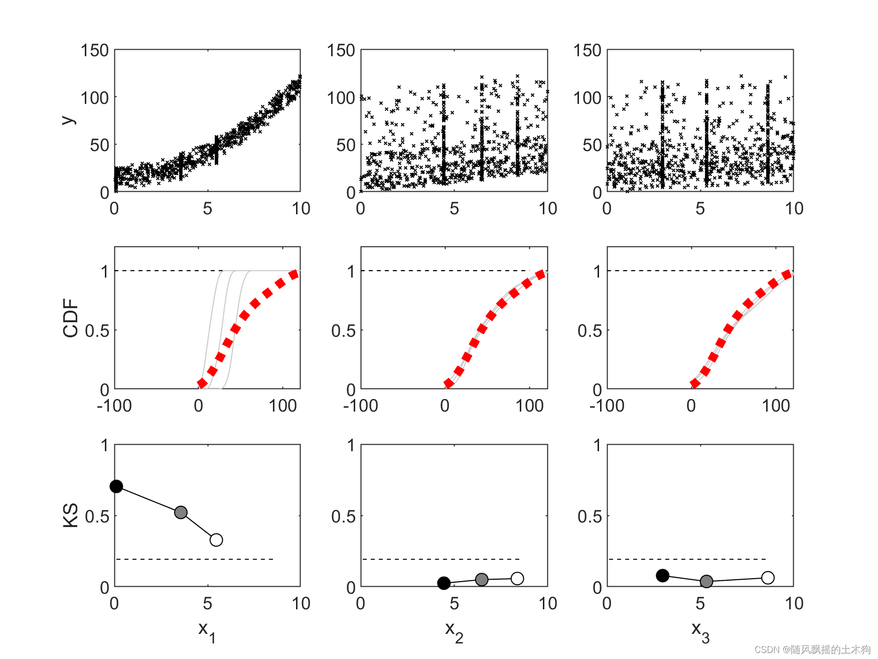
一、有条件参数
clear;

% Ishigami-Homma function
f = @(x,p) sin(x(1)) + p.a * sin(x(2)^2) + p.b * x(3)^4 * sin(x(1));
p.a = 2; p.b = 1;
ih = @(x) f(x, p);

% Bounds
lb = ones(1,3) * -pi; ub = ones(1,3) * pi;

% Parameters from Figure 4's caption
n=15;
Nu = 100;
Nc = 100; % Is actually 50 in the paper

% Other parameters
npts = 100; seed = 4;

[KS,xvals,y_u, y_c, par_u, par_c, ft] = PAWN(f, p, lb, ub, Nu, n, Nc, npts, seed);

m1 = min([y_c, y_u']);
m2 = max([y_c, y_u']);
[f,ci] = ksdensity(y_u, linspace(m1,m2,npts), 'Function', 'cdf');

% Begin Plotting
subplot(331); ylabel('y'); hold on;box on;
subplot(334); ylabel('CDF'); hold on;  box on;
subplot(337); ylabel('KS'); hold on; xlabel('x_1'); box on;
subplot(338); xlabel('x_2'); hold on;box on;
subplot(339); xlabel('x_3'); hold on;box on;
for ind=1:length(lb)
    subplot(330+ind)
    plot(par_c(:,ind),y_c, 'xk', 'markersize', 2);
end

crit_c = [1.22,1.36,1.48,1.63,1.73,1.95]; % 0.1, 0.05, 0.025, 0.010, 0.005, 0.001
critval = crit_c(2) * sqrt((Nu+Nc)/(Nu*Nc));

for ind=1:length(lb)
    subplot(333+ind)
    plot([-100, 100], [1, 1], 'k--'); hold on
    plot(ci,ft((ind-1)*n+1:ind*n,:), 'color', [0.8,0.8,0.8]); ylim([0,1]);
    plot(ci,f, 'r:','linewidth',4); ylim([0,1.2])
    hold off
end

colData = linspace(0,n,n)'/n; colData = [colData colData colData];

for ind=1:length(lb)
    subplot(336+ind)
    [xtoplot, indices] = sort(xvals(ind,:));
    ytoplot = KS(ind, :); ytoplot = ytoplot(indices);
    plot([min(xvals(:)), max(xvals(:))], [critval,critval], 'k--'); hold on;
    plot(xtoplot, ytoplot, 'k');
    scatter(xtoplot, ytoplot, [],  colData, 'filled', 'markeredgecolor', 'k');
    ylim([0,1])
    hold off
end

disp(strcat('Median of KS : ', num2str(median(KS,2)')))
disp(strcat('Max of KS : ', num2str(max(KS'))))
二、无条件参数
clear;

%目标函数
model=@(x)x(1)^2+2*x(2)+x(3)-1;

% 参数范围
lb=[0 0 0 ];%每个参数的

下限向量(1xM)
ub=[10 10 10];%每个参数的上界的向量(1xM)
% 参数设置
Nu = 100;%Nu:无条件参数空间的样本数

% 其他参数
npts = 100;%npts:用于核密度估计的点数
seed = 4;%seed:随机数种子

[y_u,  par_u ,f,ci] = PAWN(model, lb, ub, Nu, npts, seed);
%初始化

%y_u 无条件模拟的输出
 %par_u 样本生成
  %f 用核密度评估无条件样本的CDF(分布函数),表示连续型随机变量x的概率
%f返回x中样本数据的概率密度估计f。
%该估计基于正核函数,并在覆盖x中数据范围的等间距点ci处进行评估。

% Begin Plotting
figure()
subplot(231); ylabel('y'); hold on;box on;
subplot(234); ylabel('CDF'); hold on;  box on;
for ind=1:length(lb)
   subplot(230+ind)
   plot(par_u(:,ind),y_u, 'xk', 'markersize', 2);
   xlabel(['x' num2str(ind)])
end


for ind=1:length(lb)
    subplot(233+ind)
    plot([-100, 100], [1, 1], 'k--'); hold on
    plot(ci,f, 'r:','linewidth',4); ylim([0,1.2])
     xlabel(['x' num2str(ind)])
    hold off
end

三、代码获取
后台私信“66期”获取下载链接。