使用 Cox 比例风险和随机生存森林估计原发性胆汁性肝硬化患者的生存风险
欢迎来到第二门课程的最终作业!在这个作业中,你将使用生存数据以及线性和非线性技术开发风险模型。我们将使用一个包含原发性胆汁性肝硬化(pbc)患者的生存数据集。PBC 是一种由于肝内胆汁积聚(胆汁淤积)导致小胆管受损并排出肝内胆汁的疾病。
我们的目标是了解不同因素对患者的生存时间的影响。在此过程中,你将学习以下主题:
- Cox 比例风险模型、
- Cox 模型数据预处理、
- 随机生存森林
- 排列方法用于解释性。
作业解析
作业名:
Cox Proportional Hazards and Random Survival Forests.ipynb
作业地址:
github --> bharathikannann/AI-for-Medicine-Specialization-deeplearning.ai --> AI for Medical Prognosis --> Week 4
文章目录
1. 导入包
import sklearn
import numpy as np
import pandas as pd
import matplotlib.pyplot as plt

from lifelines import CoxPHFitter
from lifelines.utils import concordance_index as cindex
from sklearn.model_selection import train_test_split

from util import load_data
- sklearn 是最流行的机器学习库之一。
- numpy 是 Python 中科学计算的基本包。
- pandas 是我们用来操作数据的工具。
- matplotlib 是一个绘图库。
- lifelines 是一个开源的生存分析库。
2. 加载数据
df = load_data()
3. 探索数据
time单位为年。另外请注意,我们已经为 sex 分配了一个数值,其中 female = 0,male = 1。
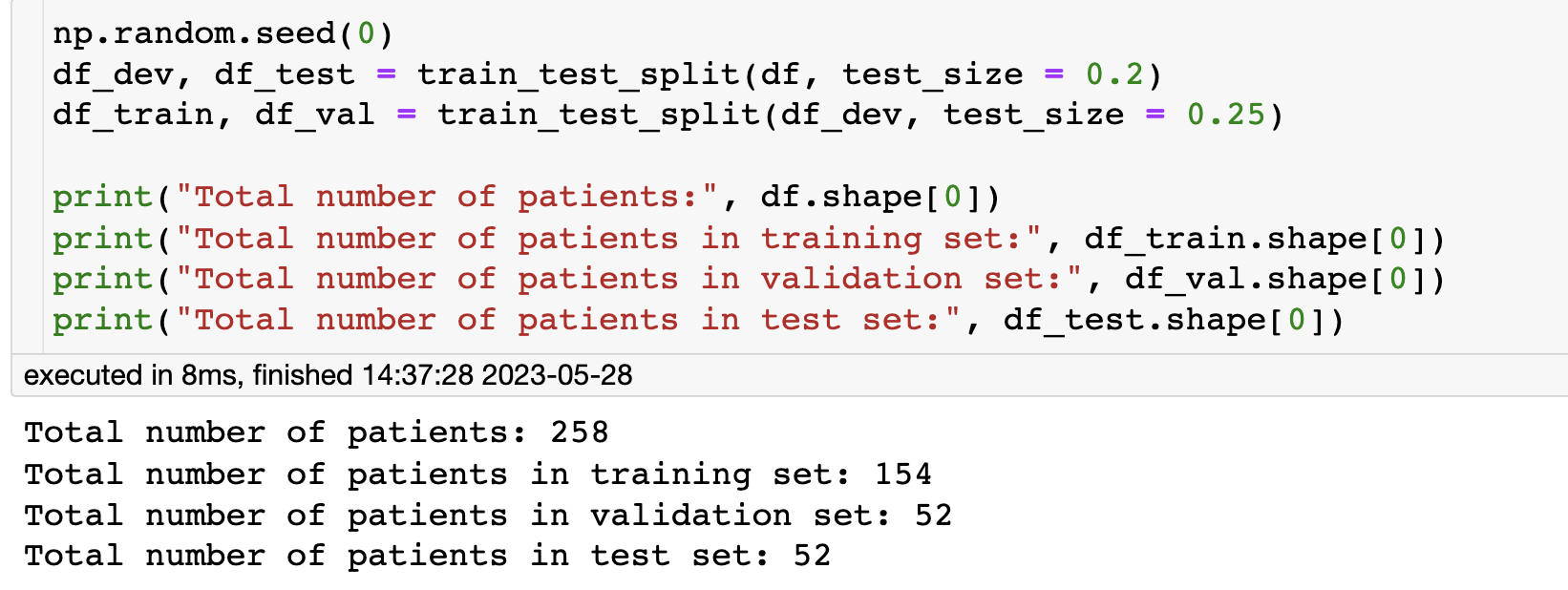
接下来,熟悉一下数据及其形状。

把数据分为训练集验证集测试集,比例为 6:2:2
在继续建模之前,让我们对连续协变量进行归一化,以确保它们在相同的尺度上。同样,我们应该使用训练数据的统计量来标准化测试数据。
continuous_columns = ['age', 'bili', 'chol', 'albumin', 'copper', 'alk.phos', 'ast', 'trig', 'platelet', 'protime']
mean = df_train.loc[:, continuous_columns].mean()
std = df_train.loc[:, continuous_columns].std()
df_train.loc[:, continuous_columns] = (df_train.loc[:, continuous_columns] - mean) / std
df_val.loc[:, continuous_columns] = (df_val.loc[:, continuous_columns] - mean) / std
df_test.loc[:, continuous_columns] = (df_test.loc[:, continuous_columns] - mean) / std
让我们检查一下训练数据集的汇总统计,以确保它是标准化的。
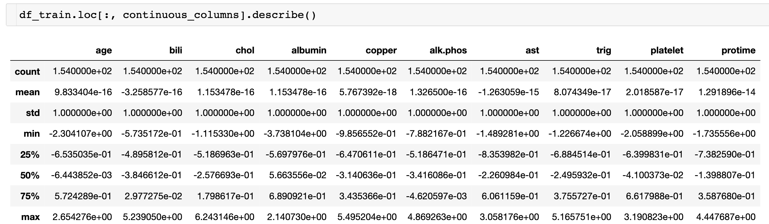
df.describe()该命令将返回Pandas数据框中数值列的计数、平均值、标准差、最小/最大值等统计信息。
4. Cox Proportional Hazards
我们的目标是使用我们拥有的生存数据构建一个风险评分。我们将从对你的数据进行Cox比例风险模型的拟合开始。
回想一下,Cox比例风险模型描述了个体 i i i在时间 t t t的危险性为:
λ ( t , x ) = λ 0 ( t ) e θ T X i \lambda(t, x) = \lambda_0(t)e^{\theta^T X_i} λ(t,x)=λ0(t)eθTXi
其中, λ 0 \lambda_0 λ0项是基准风险度,包含随着时间的推移而产生的风险,另外一个项包含由个体协变量产生的风险。在拟合模型后,我们可以使用个体相关的风险项 e θ T X i e^{\theta^T X_i} eθTXi进行排名。
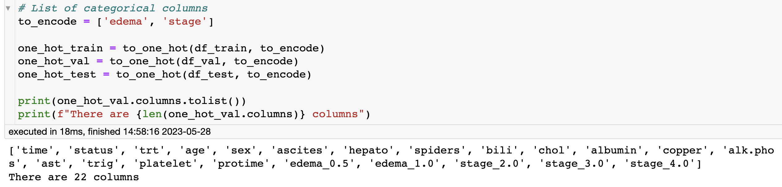
分类变量不能直接用于回归模型。为了使用它们,需要将它们转换为一系列变量。
由于我们的数据有混合的分类变量(stage)和连续性变量(wblc),因此在进一步处理之前,我们需要进行一些数据工程。为了解决这个问题,我们将使用“虚拟编码”(Dummy Coding)技术。为了使用Cox比例风险模型,我们需要将分类数据转换为one hot特征,以便我们可以拟合我们的Cox模型。幸运的是,Pandas有一个内置的名为get_dummies()函数,可以将分类特征转换为多个二进制特征,使我们更容易实现我们的功能。
Exercise 1
执行to_one_hot(...)函数
def to_one_hot(dataframe, columns):
    '''
    Convert columns in dataframe to one-hot encoding.
    Args:
        dataframe (dataframe): pandas dataframe containing covariates
        columns (list of strings): list categorical column names to one hot encode
    Returns:
        one_hot_df (dataframe): dataframe with categorical columns encoded
                            as binary variables
    '''

    ### START CODE HERE (REPLACE INSTANCES OF 'None' with your code) ###

    one_hot_df = pd.get_dummies(dataframe,columns=columns,dtype=np.float64,drop_first=True)

    ### END CODE HERE ###

    return one_hot_df
get_dummies()函数更详细的解析见上次作业
深度学习用于医学预后-第二课第四周1-4节随堂作业
5.Cox模型的拟合与可解释性
使用lifelines包拟合Cox Proportional Hazards model
cph = CoxPHFitter()
cph.fit(one_hot_train, duration_col = 'time', event_col = 'status', step_size=0.1)
注意:这里运行报错的话,是 lifelines版本不对
在 lifelines 的 0.24.0 版本和之前的版本中,CoxPHFitter 模型确实具有 step_size 参数。如果你希望使用 step_size 参数,则可以将 lifelines 库降级到此版本或更早的版本。
或者直接删掉 step_size 参数,但我删除后仍然有问题,最后,我把版本修改后正确运行
pip install lifelines==0.24.0
你可以使用 cph.print_summary() 来查看各个协变量的系数以及置信区间。
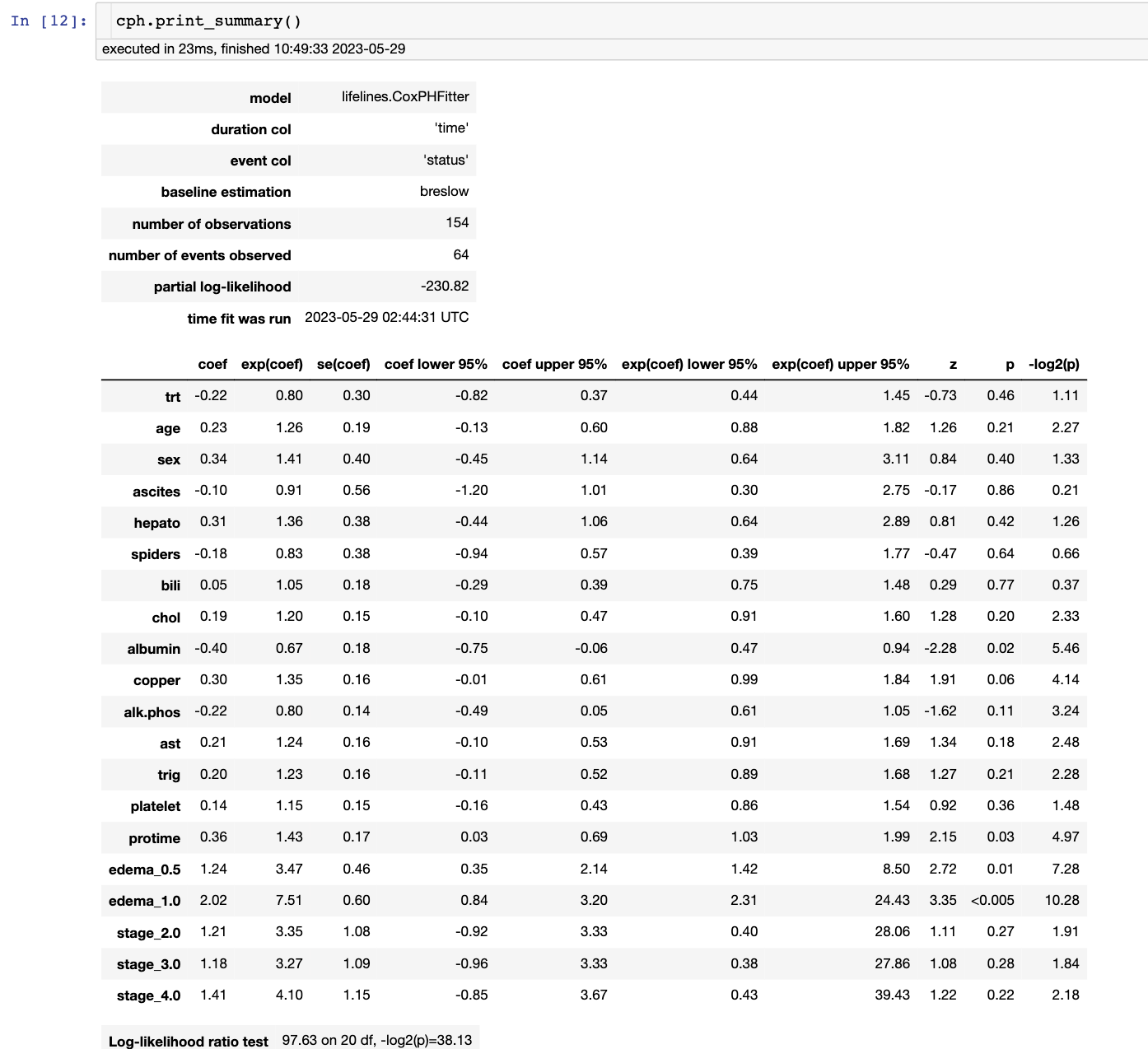
问题:
- 从模型结果来看,治疗(‘trt’参数=1,代表治疗过)是否有效?
- 它的风险比是多少?
- 需要注意的是,风险比指的是特征变量的一次增量如何改变风险。
我们可以比较‘trt’变量的预测生存曲线。运行下一个单元格,使用 plot_covariate_groups() 函数绘制生存曲线。
- y 轴是生存率
- x 轴是时间
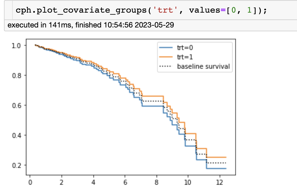
请注意,与治疗组相比,未接受治疗的组在所有时间点(x 轴是时间)的生存率都较低。
6. Hazard Ratio
回想一下课堂视频中的内容,两个病人之间的风险比是一个患者(例如吸烟者)比另一个患者(例如非吸烟者)更容易发生风险的可能性。具体来说,两个患者之间的风险比为:
λ s m o k e r ( t ) λ n o n s m o k e r ( t ) = e θ ( X s m o k e r − X n o n s m o k e r ) T \frac{\lambda_{smoker}(t)}{\lambda_{nonsmoker}(t)} = e^{\theta (X_{smoker} - X_{nonsmoker})^T} λnonsmoker(t)λsmoker(t)=eθ(Xsmoker−Xnonsmoker)T
其中,
λ s m o k e r ( t ) = λ 0 ( t ) e θ X s m o k e r T \lambda_{smoker}(t) = \lambda_0(t)e^{\theta X_{smoker}^T} λsmoker(t)=λ0(t)eθXsmokerT
λ n o n s m o k e r ( t ) = λ 0 ( t ) e θ X n o n s m o k e r T \lambda_{nonsmoker}(t) = \lambda_0(t)e^{\theta X_{nonsmoker}^T} \\ λnonsmoker(t)=λ0(t)eθXnonsmokerT
该公式表明,两个患者之间的风险比取决于 θ \theta θ 和二者之间的协变量差异 X s m o k e r − X n o n s m o k e r X_{smoker} - X_{nonsmoker} Xsmoker−Xnonsmoker。如果 θ > 0 \theta > 0 θ>0,则吸烟者的风险将高于非吸烟者,反之则低于非吸烟者。
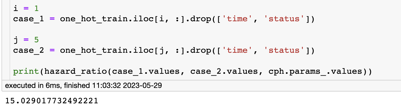
练习 2
在下面的单元格中编写一个函数,根据 Cox 模型的系数计算两个个体之间的风险比。
def hazard_ratio(case_1, case_2, cox_params):
    '''
    Return the hazard ratio of case_1 : case_2 using
    the coefficients of the cox model.

    Args:
        case_1 (np.array): (1 x d) array of covariates
        case_2 (np.array): (1 x d) array of covariates
        model (np.array): (1 x d) array of cox model coefficients
    Returns:
        hazard_ratio (float): hazard ratio of case_1 : case_2
    '''

    ### START CODE HERE (REPLACE INSTANCES OF 'None' with your code) ###

    hr = np.exp(np.dot(cox_params,(case_1 - case_2).T))

    ### END CODE HERE ###

    return hr
7. Harrell’s C-index
为了评估我们的模型表现如何,我们将编写自己版本的 C-index。类似于第一周的案例,在生存环境下,C-index 是指给定一个随机选择的两个个体,比较早死的那个是否具有更高的风险得分的概率。
然而,我们需要考虑到数据的截尾问题。想象一组病人 A A A 和 B B B。
情况 1
- A A A 的观测时间是 t A t_A tA
- B B B 在 t B t_B tB 死亡
- t A < t B t_A < t_B tA<tB.
由于存在截尾,我们无法确定 A A A 或 B B B 应该具有更高的风险得分。
情况 2
现在假设 t A > t B t_A > t_B tA>tB。
- A A A 的删失时间是 t A t_A tA
- B B B 在 t B t_B tB 死亡
- t A > t B t_A > t_B tA>tB
现在我们可以明确地说 B B B 应该比 A A A 具有更高的风险得分,因为我们确实知道 A A A 活了更长的时间。
因此,当我们计算 C-index 时:
- 我们只应考虑至多有一个被删失的个体的情况。
- 如果被删失,则他们的截尾时间应该在另一个人死亡之后出现。
如果我们使用这个规则计算得到的指标称作 Harrel’s C-index。
需要注意的是,在这种情况下,被删失意味着真实的死亡时间发生在 t t t 时间之后而不是在 t t t 时刻。
- 因此,如果 t A = t B t_A = t_B tA=tB 并且 A A A 被删失:
- 那么 A A A 实际上比 B B B 活得更长。
- 这将影响下面练习中如何处理平局的方法!
Exercise 3
to compute Harrel’s C-index.
def harrell_c(y_true, scores, event):
    '''
    Compute Harrel C-index given true event/censoring times,
    model output, and event indicators.

    Args:
        y_true (array): array of true event times
        scores (array): model risk scores
        event (array): indicator, 1 if event occurred at that index, 0 for censorship
    Returns:
        result (float): C-index metric
    '''

    n = len(y_true)
    assert (len(scores) == n and len(event) == n)

    concordant = 0.0
    permissible = 0.0
    ties = 0.0

    result = 0.0

    ### START CODE HERE (REPLACE INSTANCES OF 'None' and 'pass' with your code) ###

    # use double for loop to go through cases
    for i in range(n):
        # set lower bound on j to avoid double counting
        for j in range(i+1, n):

            # check if at most one is censored
            if event[i]==1 or event[j]==1:

                # check if neither are censored
                if event[i]==1 and event[j]==1:
                    permissible+=1
                    # check if scores are tied
                    if scores[i]==scores[j]:
                        ties = ties + 1

                    # check for concordant
                    elif scores[i]>scores[j] and y_true[i]<y_true[j]:
                        concordant = concordant + 1
                    elif scores[i]<scores[j] and y_true[j]<y_true[i]:
                        concordant = concordant + 1

                # check if one is censored
                elif event[i]==0 or event[j]==0:

                    # get censored index
                    censored = j
                    uncensored = i

                    if event[i] == 0:
                        censored = i
                        uncensored = j

                    # check if permissible
                    # Note: in this case, we are assuming that censored at a time
                    # means that you did NOT die at that time. That is, if you
                    # live until time 30 and have event = 0, then you lived THROUGH
                    # time 30.
                    if y_true[uncensored] <= y_true[censored]:
                        permissible +=1

                        # check if scores are tied
                        if scores[uncensored]==scores[censored]:
                            # update ties
                            ties = ties + 1

                        # check if scores are concordant
                        if scores[uncensored]>scores[censored]:
                            concordant = concordant + 1

    # set result to c-index computed from number of concordant pairs,
    # number of ties, and number of permissible pairs (REPLACE 0 with your code)
    result = (concordant + (0.5 * ties)) / permissible

    ### END CODE HERE ###

    return result
在我们数据上评估模型
# Train
scores = cph.predict_partial_hazard(one_hot_train)
cox_train_scores = harrell_c(one_hot_train['time'].values, scores.values, one_hot_train['status'].values)
# Validation
scores = cph.predict_partial_hazard(one_hot_val)
cox_val_scores = harrell_c(one_hot_val['time'].values, scores.values, one_hot_val['status'].values)
# Test
scores = cph.predict_partial_hazard(one_hot_test)
cox_test_scores = harrell_c(one_hot_test['time'].values, scores.values, one_hot_test['status'].values)

print("Train:", cox_train_scores)
print("Val:", cox_val_scores)
print("Test:", cox_test_scores)
- Train: 0.8265
- Val: 0.8544
- Test: 0.8478
8. Random Survival Forests
这个方法表现还不错,但你有一种预感,可以通过使用机器学习方法来提高表现。你决定使用随机生存森林(Random Survival Forest)算法。为此,你可以在 R 中使用 RandomForestSRC 软件包。为了从 Python 中调用 R 函数,我们需要使用 r2py 软件包。运行以下代码块以导入必要的需求。
这部分略,没有用过r语言,运行出了一些问题。有需要,自行下载研究吧