写在前面
- 为了保证整个示例项目更加直观,方便理解,在展示一些函数的源码时会使用numpy版本进行展示,而在示例程序中并未使用numpy版本的库,在Cython版本与numpy版本出现差异的原码前会有标注,希望读者留意。
- 3DMM实例程序的jupyter版本后续会更新,完全免费,欢迎大家下载
源码解析
在上一篇文章了解3DMM模型以及用随机的形状系数和表情系数生成面部网格进行3DMM模型的前向重建过程后进入例程的后半部分—— 由2D图像点和对应的3D顶点索引得到新的参数进而从二维图片进行三维人脸的重建。
理论部分
理论这部分借鉴了大佬的文章和一些论文。
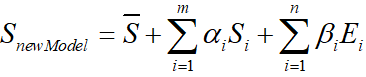
从上篇文章我们了解了3DMM模型的公式:
通过一张单张正脸照片,首先利用人脸对齐算法计算得到目标二维人脸的68个特征点坐标 x i x_i xi,在BFM模型中有对应的68个特征点 X i X_i Xi,投影后忽略第三维,则特征点之间的对应关系如下:
根据这些信息求出 α , β \alpha, \beta α,β系数,将平均脸模型与照片中的脸部进行拟合,即:
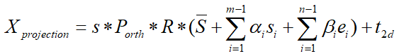
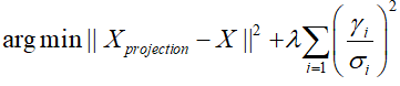
因此,三维人脸重建问题再次转化为求解系数( α , β \alpha,\beta α,β)以满足下列能量方程的问题:
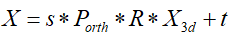
人脸模型的三维点以及对应照片中的二维点存在映射关系,这个可以由一个3x4的仿射矩阵 P P P进行表示。即: X = P A ⋅ X 3 d X=P_A\cdot X_{3d} X=PA⋅X3d。
黄金标准算法
要计算出仿射矩阵,代码中使用了黄金标准算法(Gold Standard algorithm)
算法如下:
目标为给定n>=4组3维( X i X_i Xi)到2维( x i x_i xi)的图像点对应,确定仿射摄像机投影矩阵的最大似然估计。
- 归一化,对于二维点( x i x_i xi),计算一个相似变换 T T T,使得 x ˉ = T x i \bar{x} =Tx_i xˉ=Txi,同样的对于三维点,计算 X ˉ = U X i \bar{X}=UX_i Xˉ=UXi
- 对于每组对应点 x i x_i xi~ X i X_i Xi,都有形如 A x = b A x = b Ax=b 的对应关系存在
- 求出A的伪逆
- 去掉归一化,得到仿射矩阵
在Face3d中的求解过程
过程可以概述如下:
(1)初始化 α , β \alpha,\beta α,β为0;
(2)利用黄金标准算法得到一个仿射矩阵 P A P_A PA,分解得到 s , R , t 2 d s,R,t_{2d} s,R,t2d;
(3)将(2)中求出的 s , R , t 2 d s,R,t_{2d} s,R,t2d带入能量方程,解得 α \alpha α;
(4)将(2)和(3)中求出的 α \alpha α代入能量方程,解得 β \beta β;
(5)更新 α , β \alpha,\beta α,β的值,重复(2)-(4)进行迭代更新。
代码部分
下面将从Face3D的例程到源码一步步进行讲解:
例程部分
x = projected_vertices[bfm.kpt_ind, :2] # 2d keypoint, which can be detected from image
X_ind = bfm.kpt_ind # index of keypoints in 3DMM. fixed.

# fit
fitted_sp, fitted_ep, fitted_s, fitted_angles, fitted_t = bfm.fit(x, X_ind, max_iter = 3)

# verify fitted parameters
fitted_vertices = bfm.generate_vertices(fitted_sp, fitted_ep)
transformed_vertices = bfm.transform(fitted_vertices, fitted_s, fitted_angles, fitted_t)

image_vertices = mesh.transform.to_image(transformed_vertices, h, w)
fitted_image = mesh.render.render_colors(image_vertices, bfm.triangles, colors, h, w)
x就是公式中的二维特征点 X X X,例程里面给的是上篇文章生成二维图像时导出的二维数据。
X_ind是BFM模型三维特征点的索引,并非坐标。
然后执行了
fitted_sp, fitted_ep, fitted_s, fitted_angles, fitted_t = bfm.fit(x, X_ind, max_iter = 3
其中bfm.fit部分的源码如下:
def fit(self, x, X_ind, max_iter = 4, isShow = False):
        ''' fit 3dmm & pose parameters
        Args:
            x: (n, 2) image points
            X_ind: (n,) corresponding Model vertex indices
            max_iter: iteration
            isShow: whether to reserve middle results for show
        Returns:
            fitted_sp: (n_sp, 1). shape parameters
            fitted_ep: (n_ep, 1). exp parameters
            s, angles, t
        '''
        if isShow:
            fitted_sp, fitted_ep, s, R, t = fit.fit_points_for_show(x, X_ind, self.model, n_sp = self.n_shape_para, n_ep = self.n_exp_para, max_iter = max_iter)
            angles = np.zeros((R.shape[0], 3))
            for i in range(R.shape[0]):
                angles[i] = mesh.transform.matrix2angle(R[i])
        else:
            fitted_sp, fitted_ep, s, R, t = fit.fit_points(x, X_ind, self.model, n_sp = self.n_shape_para, n_ep = self.n_exp_para, max_iter = max_iter)
            angles = mesh.transform.matrix2angle(R)
        return fitted_sp, fitted_ep, s, angles, t
标签isShow给的是默认的False所以执行的else部分,里面执行了模型拟合部分代码:
fitted_sp, fitted_ep, s, R, t = fit.fit_points(x, X_ind, self.model, n_sp = self.n_shape_para, n_ep = self.n_exp_para, max_iter = max_iter)
以及生成旋转矩阵代码:
angles = mesh.transform.matrix2angle(R)
其中模型拟合部分的fit.fit_points部分的源码如下:
def fit_points(x, X_ind, model, n_sp, n_ep, max_iter = 4):
    '''
    Args:
        x: (n, 2) image points
        X_ind: (n,) corresponding Model vertex indices
        model: 3DMM
        max_iter: iteration
    Returns:
        sp: (n_sp, 1). shape parameters
        ep: (n_ep, 1). exp parameters
        s, R, t
    '''
    x = x.copy().T

    #-- init
    sp = np.zeros((n_sp, 1), dtype = np.float32)
    ep = np.zeros((n_ep, 1), dtype = np.float32)

    #-------------------- estimate
    X_ind_all = np.tile(X_ind[np.newaxis, :], [3, 1])*3
    X_ind_all[1, :] += 1
    X_ind_all[2, :] += 2
    valid_ind = X_ind_all.flatten('F')

    shapeMU = model['shapeMU'][valid_ind, :]
    shapePC = model['shapePC'][valid_ind, :n_sp]
    expPC = model['expPC'][valid_ind, :n_ep]

    for i in range(max_iter):
        X = shapeMU + shapePC.dot(sp) + expPC.dot(ep)
        X = np.reshape(X, [int(len(X)/3), 3]).T

        #----- estimate pose
        P = mesh.transform.estimate_affine_matrix_3d22d(X.T, x.T)
        s, R, t = mesh.transform.P2sRt(P)
        rx, ry, rz = mesh.transform.matrix2angle(R)
        # print('Iter:{}; estimated pose: s {}, rx {}, ry {}, rz {}, t1 {}, t2 {}'.format(i, s, rx, ry, rz, t[0], t[1]))

        #----- estimate shape
        # expression
        shape = shapePC.dot(sp)
        shape = np.reshape(shape, [int(len(shape)/3), 3]).T
        ep = estimate_expression(x, shapeMU, expPC, model['expEV'][:n_ep,:], shape, s, R, t[:2], lamb = 0.002)

        # shape
        expression = expPC.dot(ep)
        expression = np.reshape(expression, [int(len(expression)/3), 3]).T
        sp = estimate_shape(x, shapeMU, shapePC, model['shapeEV'][:n_sp,:], expression, s, R, t[:2], lamb = 0.004)

    return sp, ep, s, R, t
fit.fit_points部分拆分讲解
(1)初始化 α , β \alpha,\beta α,β为0
x = x.copy().T

    #-- init
    sp = np.zeros((n_sp, 1), dtype = np.float32)
    ep = np.zeros((n_ep, 1), dtype = np.float32)
x取转置,格式变为(2,68)
sp即 α \alpha α,ep即 β \beta β。将它们赋值为格式(199,1)的零向量。
- X 3 d X_{3d} X3d进行坐标转换
由于BFM模型中的顶点坐标储存格式为{ x 1 x_1 x1, y 1 y_1 y1, z 1 z_1 z1, x 2 x_2 x2, y 2 y_2 y2, z 2 z_2 z2, x 3 x_3 x3, y 3 y_3 y3,…}
而在X_ind中只给出了三位特征点坐标的位置,所以应该根据X_ind获取 X 3 d X_{3d} X3d的XYZ坐标数据。
X_ind_all = np.tile(X_ind[np.newaxis, :], [3, 1])*3
    X_ind_all[1, :] += 1
    X_ind_all[2, :] += 2
    valid_ind = X_ind_all.flatten('F')
X_ind数据如下,是一个(68,1)的位置数据。
X_ind_all = np.tile(X_ind[np.newaxis, :], [3, 1])*3
X_ind_all拓展为(3,68)并乘3来定位到坐标位置:

X_ind_all[1, :] += 1
X_ind_all[2, :] += 2
再将第二行加一、第三行加二来对于Y坐标和Z坐标。

然后将它们合并
valid_ind = X_ind_all.flatten('F')
flatten是numpy.ndarray.flatten的一个函数,即返回一个折叠成一维的数组。但是该函数只能适用于numpy对象,即array或者mat,普通的list列表是不行的。
'F’表示以列优先展开。
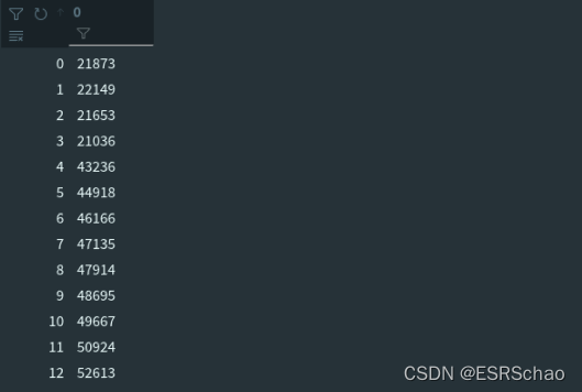
合并后的结果valid_ind如下图:

通过合并后的valid_ind得到对应特征点的人脸形状、形状主成分、表情主成分这三种数据。
shapeMU = model['shapeMU'][valid_ind, :]
shapePC = model['shapePC'][valid_ind, :n_sp]
expPC = model['expPC'][valid_ind, :n_ep]
人脸形状shapeMU数据格式(68*3,1)
形状主成分shapePC数据格式(68*3,199)
表情主成分expPC数据格式(68*3,29)
for i in range(max_iter):
        X = shapeMU + shapePC.dot(sp) + expPC.dot(ep)
        X = np.reshape(X, [int(len(X)/3), 3]).T

        #----- estimate pose
        P = mesh.transform.estimate_affine_matrix_3d22d(X.T, x.T)
        s, R, t = mesh.transform.P2sRt(P)
        rx, ry, rz = mesh.transform.matrix2angle(R)
        # print('Iter:{}; estimated pose: s {}, rx {}, ry {}, rz {}, t1 {}, t2 {}'.format(i, s, rx, ry, rz, t[0], t[1]))

        #----- estimate shape
        # expression
        shape = shapePC.dot(sp)
        shape = np.reshape(shape, [int(len(shape)/3), 3]).T
        ep = estimate_expression(x, shapeMU, expPC, model['expEV'][:n_ep,:], shape, s, R, t[:2], lamb = 0.002)

        # shape
        expression = expPC.dot(ep)
        expression = np.reshape(expression, [int(len(expression)/3), 3]).T
        sp = estimate_shape(x, shapeMU, shapePC, model['shapeEV'][:n_sp,:], expression, s, R, t[:2], lamb = 0.004)

    return sp, ep, s, R, t
循环中的max_iter是自行定义的迭代次数,这里的输入为4。
X = shapeMU + shapePC.dot(sp) + expPC.dot(ep)
X = np.reshape(X, [int(len(X)/3), 3]).T
这里的 X X X就是经过如下的运算的 S n e w m o d e l S_{newmodel} Snewmodel,就是新的 X 3 d X_{3d} X3d。

真正重点的是mesh.transform.estimate_affine_matrix_3d22d(X.T, x.T),这是网格的拟合部分。
源码如下:
estimate_affine_matrix_3d22d(X, x):
    ''' Using Golden Standard Algorithm for estimating an affine camera
        matrix P from world to image correspondences.
        See Alg.7.2. in MVGCV
        Code Ref: https://github.com/patrikhuber/eos/blob/master/include/eos/fitting/affine_camera_estimation.hpp
        x_homo = X_homo.dot(P_Affine)
    Args:
        X: [n, 3]. corresponding 3d points(fixed)
        x: [n, 2]. n>=4. 2d points(moving). x = PX
    Returns:
        P_Affine: [3, 4]. Affine camera matrix
    '''
    X = X.T; x = x.T
    assert(x.shape[1] == X.shape[1])
    n = x.shape[1]
    assert(n >= 4)

    #--- 1. normalization
    # 2d points
    mean = np.mean(x, 1) # (2,)
    x = x - np.tile(mean[:, np.newaxis], [1, n])
    average_norm = np.mean(np.sqrt(np.sum(x**2, 0)))
    scale = np.sqrt(2) / average_norm
    x = scale * x

    T = np.zeros((3,3), dtype = np.float32)
    T[0, 0] = T[1, 1] = scale
    T[:2, 2] = -mean*scale
    T[2, 2] = 1

    # 3d points
    X_homo = np.vstack((X, np.ones((1, n))))
    mean = np.mean(X, 1) # (3,)
    X = X - np.tile(mean[:, np.newaxis], [1, n])
    m = X_homo[:3,:] - X
    average_norm = np.mean(np.sqrt(np.sum(X**2, 0)))
    scale = np.sqrt(3) / average_norm
    X = scale * X

    U = np.zeros((4,4), dtype = np.float32)
    U[0, 0] = U[1, 1] = U[2, 2] = scale
    U[:3, 3] = -mean*scale
    U[3, 3] = 1

    # --- 2. equations
    A = np.zeros((n*2, 8), dtype = np.float32);
    X_homo = np.vstack((X, np.ones((1, n)))).T
    A[:n, :4] = X_homo
    A[n:, 4:] = X_homo
    b = np.reshape(x, [-1, 1])

    # --- 3. solution
    p_8 = np.linalg.pinv(A).dot(b)
    P = np.zeros((3, 4), dtype = np.float32)
    P[0, :] = p_8[:4, 0]
    P[1, :] = p_8[4:, 0]
    P[-1, -1] = 1

    # --- 4. denormalization
    P_Affine = np.linalg.inv(T).dot(P.dot(U))
    return P_Affine

def P2sRt(P):
    ''' decompositing camera matrix P
    Args:
        P: (3, 4). Affine Camera Matrix.
    Returns:
        s: scale factor.
        R: (3, 3). rotation matrix.
        t: (3,). translation.
    '''
    t = P[:, 3]
    R1 = P[0:1, :3]
    R2 = P[1:2, :3]
    s = (np.linalg.norm(R1) + np.linalg.norm(R2))/2.0
    r1 = R1/np.linalg.norm(R1)
    r2 = R2/np.linalg.norm(R2)
    r3 = np.cross(r1, r2)

    R = np.concatenate((r1, r2, r3), 0)
    return s, R, t
下面对这部分进行详细解读。
(2) 利用黄金标准算法得到一个仿射矩阵 P A P_A PA,分解得到 s , R , t 2 d s,R,t_{2d} s,R,t2d;
estimate_affine_matrix_3d22d部分即黄金标准算法具体过程
a) 归一化
对于二维点 X X X,计算一个相似变换 T T T,使得 X ˉ = T X \bar{X}=TX Xˉ=TX,同样的对于三维点 X 3 d X_{3d} X3d,计算 X ˉ 3 d = U X 3 d \bar{X}_{3d}=UX_{3d} Xˉ3d=UX3d。
归一化部分的概念在Multiple View Geometry in Computer Vision一书中描述如下:
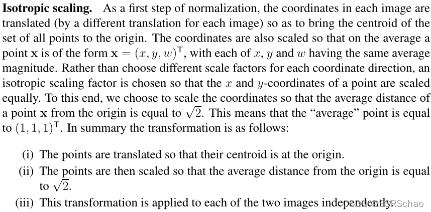 所以归一化可以概述为以下三步:
- 平移所有坐标点,使它们的质心位于原点。
- 然后对这些点进行缩放,使到原点的平均距离等于 2 \sqrt{2} 2。
- 将该变换应用于图像中的每一幅。
下面结合代码进行讲解:
输入检测,确保输入的二维和三维特征点的数目一致以及特征点数目大于4。
 X = X.T; x = x.T
    assert(x.shape[1] == X.shape[1])
    n = x.shape[1]
    assert(n >= 4)
二维数据归一化:
    #--- 1. normalization
    # 2d points
    mean = np.mean(x, 1) # (2,)
    x = x - np.tile(mean[:, np.newaxis], [1, n])
    average_norm = np.mean(np.sqrt(np.sum(x**2, 0)))
    scale = np.sqrt(2) / average_norm
    x = scale * x

    T = np.zeros((3,3), dtype = np.float32)
    T[0, 0] = T[1, 1] = scale
    T[:2, 2] = -mean*scale
    T[2, 2] = 1
- 平移所有坐标点,使它们的质心位于原点。
经过x=x.T后x的格式变为(2,68)
通过mean = np.mean(x, 1)获取x的X坐标和Y坐标平均值mean,格式为(2,)
这一步x = x - np.tile(mean[:, np.newaxis], [1, n])
x的所有XY坐标都减去刚刚算出的平均值,此时x中的坐标点被平移到了质心位于原点的位置。 - 然后对这些点进行缩放,使到原点的平均距离等于 2 \sqrt{2} 2。
average_norm = np.mean(np.sqrt(np.sum(x**2, 0)))
算出所有此时所有二维点到原点的平均距离average_norm,这是一个数值。
scale = np.sqrt(2) / average_norm
x = scale * x
算出scale再用scale去乘x坐标,相当与x所有的坐标除以当前的平均距离之后乘以 2 \sqrt{2} 2。
这样算出来的所有点到原点的平均距离就被缩放到了 2 \sqrt{2} 2。 - 同时通过计算出的scale和mean可以算出相似变换T
T = np.zeros((3,3), dtype = np.float32)
T[0, 0] = T[1, 1] = scale
T[:2, 2] = -mean*scale
T[2, 2] = 1
# 3d points
    X_homo = np.vstack((X, np.ones((1, n))))
    mean = np.mean(X, 1) # (3,)
    X = X - np.tile(mean[:, np.newaxis], [1, n])
    m = X_homo[:3,:] - X
    average_norm = np.mean(np.sqrt(np.sum(X**2, 0)))
    scale = np.sqrt(3) / average_norm
    X = scale * X

    U = np.zeros((4,4), dtype = np.float32)
    U[0, 0] = U[1, 1] = U[2, 2] = scale
    U[:3, 3] = -mean*scale
    U[3, 3] = 1
三位归一化的原理与二维相似,区别就是所有点到原点的平均距离要被缩放到 3 \sqrt{3} 3,以及生成的相似变换矩阵 U U U格式为(4,4)。这里不赘述了。
b) 对于每组对应点 x i x_i xi~ X i X_i Xi,都有形如 A x = b A x = b Ax=b 的对应关系存在
# --- 2. equations
    A = np.zeros((n*2, 8), dtype = np.float32);
    X_homo = np.vstack((X, np.ones((1, n)))).T
    A[:n, :4] = X_homo
    A[n:, 4:] = X_homo
    b = np.reshape(x, [-1, 1])
这里结合下面的公式来看:
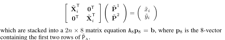 A对应其中的 [ X ˉ i T 0 T 0 T X i T ] \left [\begin{array}{l} \bar{X}_i^T & 0^T\\0^T & {X}_i^T\end{array}\right ] [XˉiT0T0TXiT]
b是展开为(68*2,1)格式的x。
c) 求出A的伪逆
 # --- 3. solution
    p_8 = np.linalg.pinv(A).dot(b)
    P = np.zeros((3, 4), dtype = np.float32)
    P[0, :] = p_8[:4, 0]
    P[1, :] = p_8[4:, 0]
    P[-1, -1] = 1
关于A的伪逆的概念和求取方法可以参照Multiple View Geometry in Computer Vision书中的P590以后的内容。这里A的伪逆是利用numpy里面的函数np.linalg.pinv直接计算出来的,非常方便。
d)去掉归一化,得到仿射矩阵
 # --- 4. denormalization
    P_Affine = np.linalg.inv(T).dot(P.dot(U))
    return P_Affine
这部分的代码参照公式:
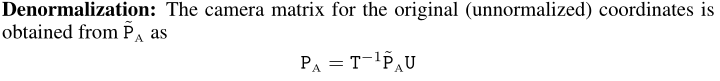
以上四步就是黄金标准算法的完整过程
得到的 P A f f i n e P_{Affine} PAffine就是式中的 P A P_A PA,到这里,我们通过黄金标准算法得到了 X = P A ⋅ X 3 d X=P_A\cdot X_{3d} X=PA⋅X3d中的 P A P_A PA。
将仿射矩阵 R A R_A RA分解得到 s , R , t 2 d s,R,t_{2d} s,R,t2d
s, R, t = mesh.transform.P2sRt(P)
rx, ry, rz = mesh.transform.matrix2angle(R)
其中mesh.transform.P2sRt部分的源码如下:
def P2sRt(P):
    ''' decompositing camera matrix P
    Args:
        P: (3, 4). Affine Camera Matrix.
    Returns:
        s: scale factor.
        R: (3, 3). rotation matrix.
        t: (3,). translation.
    '''
    t = P[:, 3]
    R1 = P[0:1, :3]
    R2 = P[1:2, :3]
    s = (np.linalg.norm(R1) + np.linalg.norm(R2))/2.0
    r1 = R1/np.linalg.norm(R1)
    r2 = R2/np.linalg.norm(R2)
    r3 = np.cross(r1, r2)

    R = np.concatenate((r1, r2, r3), 0)
    return s, R, t
这部分就是将仿射矩阵 R A {R_A} RA分解为下图的缩放比例s、旋转矩阵R以及平移矩阵t。
这部分代码比较简单,读者可以自行理解。
篇幅原因,这边只给出(1)(2)的源码解析部分,求解 α , β \alpha,\beta α,β的过程将在下篇文章讲解。