论文速读 – SalsaNet: Fast Road and Vehicle Segmentation in LiDAR Point Clouds for Autonomous Driving

介绍：
本文主要描述了关于激光点云在自动驾驶领域语义分割的网络，主要分割路面与车辆。网络结构简单移动，原文源码版本是tensorflow版本，源码清晰简单易懂。后期升级版SalsaNext也会奉上，喜欢的同学给点个赞吧，您的支持是我更新的最大动力！
在这里插入图片描述
参考：
1.【论文阅读】SalsaNet+SalsaNext
2. salsaNet
3. resnet shortcut抄近道

一. SalsaNet

1. 主要工作

介绍了一种编码器-解码器体系结构，用于实时语义分割，针对道路和车辆点。
自动标注3D激光雷达点云，从其他传感器模态标注结果转换标签
研究了两种常用的点云投影方法BEV, FSV及其在语义上的效果，比较准确性和速度。
Kitti 数据集提出了定量比价与其他sota网络。

2. 方法

2.1 自动化数据标注

在这里插入图片描述
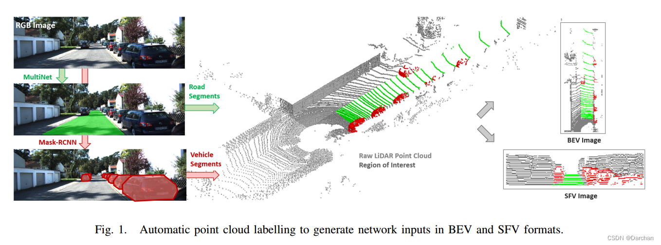
MultiNet：图像地面分割，得到地面标签
MaskRCNN：图像车辆分割，得到车辆标签
最后利用camera-lidar外参文件，对BEV和SFV image，标记出对应点云。个人理解是将点云投影到图像上，把图像上对应标签的点云赋予标签即可。

2.2 点云表征

BEV：鸟瞰图，编码4通道信息，包含每个cell平均高度、最大高度、平均强度、点数。高度最小值和std，实验证明没贡献，实验证明此输入模型效果更好。
SFV：前视图，把点云组成uv坐标系。需要编码的内容包括3d坐标系下的坐标、强度值i、范围r以及一个用于表示是否被占用的掩码，相当于变成了6通道的输入。

2.3 网络结构与源码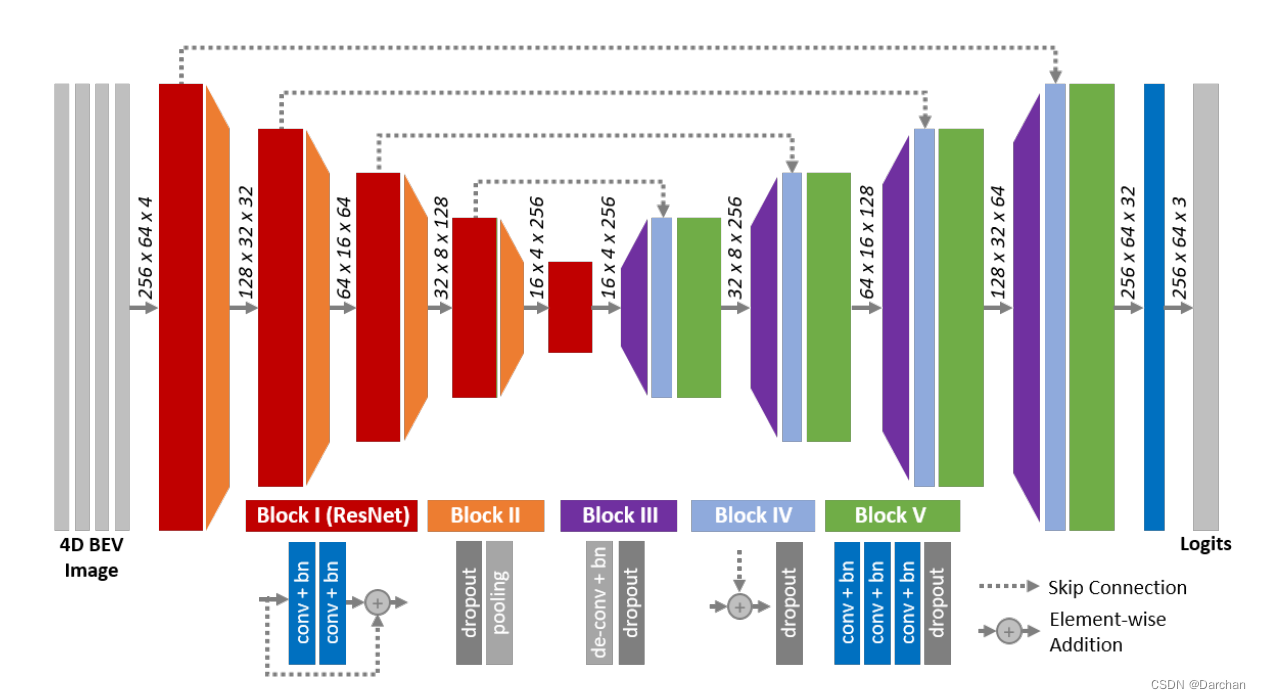

网络的源码结构：

    ## encoder
    down0c, down0b = resBlock(input_img, filter_nbr=kernel_number, dropout_rate=dropout_rate, kernel_size=3, stride=1, layer_name="res0", training=is_training, repetition=1)
    down1c, down1b = resBlock(down0c, filter_nbr=2 * kernel_number, dropout_rate=dropout_rate, kernel_size=3, stride=1, layer_name="res1", training=is_training, repetition=1)
    down2c, down2b = resBlock(down1c, filter_nbr=4 * kernel_number, dropout_rate=dropout_rate, kernel_size=3, stride=1, layer_name="res2", training=is_training, repetition=1)
    down3c, down3b = resBlock(down2c, filter_nbr=8 * kernel_number, dropout_rate=dropout_rate, kernel_size=3, stride=1, layer_name="res3", training=is_training, repetition=1)
    down4b = resBlock(down3c, filter_nbr=8 * kernel_number, dropout_rate=dropout_rate, kernel_size=3, stride=1, layer_name="res4", training=is_training, pooling=False, repetition=1)
    
    ## decoder
    up3e = upBlock(down4b, down3b,  filter_nbr=8 * kernel_number, dropout_rate=dropout_rate, kernel_size=(3, 3), layer_name="up3", training=is_training)
    up2e = upBlock(up3e, down2b,  filter_nbr=4 * kernel_number, dropout_rate=dropout_rate, kernel_size=(3, 3), layer_name="up2", training=is_training)
    up1e = upBlock(up2e, down1b,  filter_nbr=2 * kernel_number, dropout_rate=dropout_rate, kernel_size=(3, 3), layer_name="up1", training=is_training)
    up0e = upBlock(up1e, down0b,  filter_nbr= kernel_number, dropout_rate=dropout_rate, kernel_size=(3, 3), layer_name="up0", training=is_training)

    with tf.variable_scope('logits'):
        logits = conv2d_layer(up0e, num_classes, [1, 1], activation_fn=None)
        print("logits", logits.shape.as_list())

    return logits

encoder
使用的是残差块ResNet，并且除了最后一个残差块，每个残差块后都跟着一个dropout和池化组成的子模块，其中池化采用的是2×2大小的最大池化，经过四次的子模块，将feature map的大小缩小一共16倍，与此同时通道数目也增加64倍。

def resBlock(input_layer, filter_nbr, dropout_rate, kernel_size=(3, 3), stride=1, layer_name="rb", training=True,
             pooling=True, repetition=1):
    with tf.variable_scope(layer_name):

        resA = input_layer

        for i in range(repetition):
            shortcut = conv2d_layer(resA, filter_nbr, kernel_size=(1, 1), stride=stride, activation_fn=leakyRelu,
                                    scope=layer_name + '_s_%d' % (i + 0))

            resA = conv2d_layer(resA, filter_nbr, kernel_size, normalizer_fn=batchnorm,
                                activation_fn=leakyRelu,
                                normalizer_params={'is_training': training},
                                scope=layer_name + '_%d_conv1' % (i + 0))

            resA = conv2d_layer(resA, filter_nbr, kernel_size, normalizer_fn=batchnorm,
                                activation_fn=leakyRelu,
                                normalizer_params={'is_training': training},
                                scope=layer_name + '_%d_conv2' % (i + 0))

            resA = tf.add(resA, shortcut)

        if pooling:
            resB = dropout_layer(resA, rate=dropout_rate, name="dropout")
            resB = maxpool_layer(resB, (2, 2), padding='same')

            print(str(layer_name) + str(resB.shape.as_list()))
            return resB, resA
        else:
            resB = dropout_layer(resA, rate=dropout_rate, name="dropout")
            print(str(layer_name) + str(resB.shape.as_list()))
            return resB

decoder
由三个小模块组成.

第一个小模块: deconv+bn+leakyRelu+ dropoutput
第二个小模块: shortcut+dropout
第三个小模块：三个conv+bn+leakyRelu+dropout

def upBlock(input_layer, skip_layer, filter_nbr, dropout_rate, kernel_size=(3, 3), layer_name="dec", training=True):
    with tf.variable_scope(layer_name + "_up"):
        upA = conv2d_trans_layer(input_layer, filter_nbr, kernel_size, 2, normalizer_fn=batchnorm,
                                 activation_fn=leakyRelu,
                                 normalizer_params={'is_training': training}, scope="tconv")
        upA = dropout_layer(upA, rate=dropout_rate, name="dropout")

    with tf.variable_scope(layer_name + "_add"):
        upB = tf.add(upA, skip_layer, name="add")
        upB = dropout_layer(upB, rate=dropout_rate, name="dropout_add")

    with tf.variable_scope(layer_name + "_conv"):
        upE = conv2d_layer(upB, filter_nbr, kernel_size, normalizer_fn=batchnorm,
                           activation_fn=leakyRelu,
                           normalizer_params={'is_training': training}, scope="conv1")
        upE = conv2d_layer(upE, filter_nbr, kernel_size, normalizer_fn=batchnorm,
                           activation_fn=leakyRelu,
                           normalizer_params={'is_training': training}, scope="conv2")
        upE = conv2d_layer(upE, filter_nbr, kernel_size, normalizer_fn=batchnorm,
                           activation_fn=leakyRelu,
                           normalizer_params={'is_training': training}, scope="conv3")
        upE = dropout_layer(upE, rate=dropout_rate, name="dropout_conv")

        print(str(layer_name) + str(upE.shape.as_list()))

        return upE

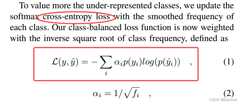
2.4 类平衡loss

数据集类型不平衡对网络性能的影响，如果按照一般的网络进行训练，对这种类别的判断会产生不好的影响，因此论文修改了损失函数的写法，引入一个权值的项，以此保证出现少的类别也能够有足够的影响力。
在这里插入图片描述

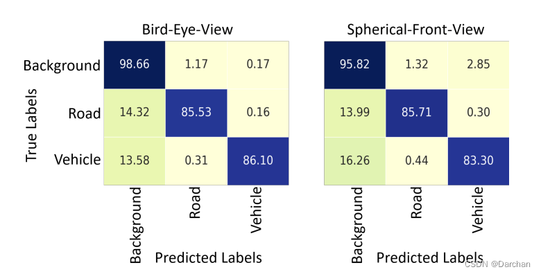
3. 结果

在这里插入图片描述