Coursera深度学习课程 DeepLearning.ai 编程作业——Building your Recurrent Neural Network - Step by Step

Building your Recurrent Neural Network - Step by Step

Welcome to Course 5’s first assignment! In this assignment, you will implement your first Recurrent Neural Network in numpy.

Recurrent Neural Networks (RNN) are very effective for Natural Language Processing and other sequence tasks because they have “memory”. They can read inputs $x^{\langle t \rangle}$ (such as words) one at a time, and remember some information/context through the hidden layer activations that get passed from one time-step to the next. This allows a uni-directional RNN to take information from the past to process later inputs. A bidirection RNN can take context from both the past and the future.

Notation:
- Superscript $[l]$ denotes an object associated with the $l^{th}$ layer. ($[l]$表示第$l^{th}$层)
- Example: $a^{[4]}$ is the $4^{th}$ layer activation. $W^{[5]}$ and $b^{[5]}$ are the $5^{th}$ layer parameters.

• Superscript $(i)$ denotes an object associated with the $i^{th}$ example. ($(i)$ 表示第 $i$ 个样本)

  • Example: $x^{(i)}$ is the $i^{th}$ training example input.

• Superscript $\langle t \rangle$ denotes an object at the $t^{th}$ time-step. （$\langle t \rangle$表示第t个时间段）

  • Example: $x^{\langle t \rangle}$ is the input x at the $t^{th}$ time-step. $x^{(i)\langle t \rangle}$ is the input at the $t^{th}$ timestep of example $i$.

• Lowerscript $i$ denotes the $i^{th}$ entry of a vector. （$a^{[l]}_i$ 表示层数激活层的第$i^{th}$个输入 ）

  • Example: $a^{[l]}_i$ denotes the $i^{th}$ entry of the activations in layer $l$.

We assume that you are already familiar with numpy and/or have completed the previous courses of the specialization. Let’s get started!

rnn_utils.py

import numpy as np

def softmax(x):
    e_x = np.exp(x - np.max(x))
    return e_x / e_x.sum(axis=0)

def smooth(loss, cur_loss):
    return loss * 0.999 + cur_loss * 0.001

def print_sample(sample_ix, ix_to_char):
    txt = ''.join(ix_to_char[ix] for ix in sample_ix)
    print ('----\n %s \n----' % (txt, ))

def get_initial_loss(vocab_size, seq_length):
    return -np.log(1.0/vocab_size)*seq_length

def softmax(x):
    e_x = np.exp(x - np.max(x))
    return e_x / e_x.sum(axis=0)

def initialize_parameters(n_a, n_x, n_y):
    """
    Initialize parameters with small random values

    Returns:
    parameters -- python dictionary containing:
                        Wax -- Weight matrix multiplying the input, numpy array of shape (n_a, n_x)
                        Waa -- Weight matrix multiplying the hidden state, numpy array of shape (n_a, n_a)
                        Wya -- Weight matrix relating the hidden-state to the output, numpy array of shape (n_y, n_a)
                        b --  Bias, numpy array of shape (n_a, 1)
                        by -- Bias relating the hidden-state to the output, numpy array of shape (n_y, 1)
    """
    np.random.seed(1)
    Wax = np.random.randn(n_a, n_x)*0.01 # input to hidden
    Waa = np.random.randn(n_a, n_a)*0.01 # hidden to hidden
    Wya = np.random.randn(n_y, n_a)*0.01 # hidden to output
    b = np.zeros((n_a, 1)) # hidden bias
    by = np.zeros((n_y, 1)) # output bias

    parameters = {"Wax": Wax, "Waa": Waa, "Wya": Wya, "b": b,"by": by}

    return parameters

def rnn_step_forward(parameters, a_prev, x):

    Waa, Wax, Wya, by, b = parameters['Waa'], parameters['Wax'], parameters['Wya'], parameters['by'], parameters['b']
    a_next = np.tanh(np.dot(Wax, x) + np.dot(Waa, a_prev) + b) # hidden state
    p_t = softmax(np.dot(Wya, a_next) + by) # unnormalized log probabilities for next chars # probabilities for next chars 

    return a_next, p_t

def rnn_step_backward(dy, gradients, parameters, x, a, a_prev):

    gradients['dWya'] += np.dot(dy, a.T)
    gradients['dby'] += dy
    da = np.dot(parameters['Wya'].T, dy) + gradients['da_next'] # backprop into h
    daraw = (1 - a * a) * da # backprop through tanh nonlinearity
    gradients['db'] += daraw
    gradients['dWax'] += np.dot(daraw, x.T)
    gradients['dWaa'] += np.dot(daraw, a_prev.T)
    gradients['da_next'] = np.dot(parameters['Waa'].T, daraw)
    return gradients

def update_parameters(parameters, gradients, lr):

    parameters['Wax'] += -lr * gradients['dWax']
    parameters['Waa'] += -lr * gradients['dWaa']
    parameters['Wya'] += -lr * gradients['dWya']
    parameters['b']  += -lr * gradients['db']
    parameters['by']  += -lr * gradients['dby']
    return parameters

def rnn_forward(X, Y, a0, parameters, vocab_size = 71):

    # Initialize x, a and y_hat as empty dictionaries
    x, a, y_hat = {}, {}, {}

    a[-1] = np.copy(a0)

    # initialize your loss to 0
    loss = 0

    for t in range(len(X)):

        # Set x[t] to be the one-hot vector representation of the t'th character in X.
        x[t] = np.zeros((vocab_size,1)) 
        x[t][X[t]] = 1

        # Run one step forward of the RNN
        a[t], y_hat[t] = rnn_step_forward(parameters, a[t-1], x[t])

        # Update the loss by substracting the cross-entropy term of this time-step from it.
        loss -= np.log(y_hat[t][Y[t],0])

    cache = (y_hat, a, x)

    return loss, cache

def rnn_backward(X, Y, parameters, cache):
    # Initialize gradients as an empty dictionary
    gradients = {}

    # Retrieve from cache and parameters
    (y_hat, a, x) = cache
    Waa, Wax, Wya, by, b = parameters['Waa'], parameters['Wax'], parameters['Wya'], parameters['by'], parameters['b']

    # each one should be initialized to zeros of the same dimension as its corresponding parameter
    gradients['dWax'], gradients['dWaa'], gradients['dWya'] = np.zeros_like(Wax), np.zeros_like(Waa), np.zeros_like(Wya)
    gradients['db'], gradients['dby'] = np.zeros_like(b), np.zeros_like(by)
    gradients['da_next'] = np.zeros_like(a[0])

    ### START CODE HERE ###
    # Backpropagate through time
    for t in reversed(range(len(X))):
        dy = np.copy(y_hat[t])
        dy[Y[t]] -= 1
        gradients = rnn_step_backward(dy, gradients, parameters, x[t], a[t], a[t-1])
    ### END CODE HERE ###

    return gradients, a

Let’s first import all the packages that you will need during this assignment.

import numpy as np
from rnn_utils import *

1 - Forward propagation for the basic Recurrent Neural Network

Later this week, you will generate music using an RNN. The basic RNN that you will implement has the structure below. In this example, $T_x = T_y$.

Figure 1: Basic RNN model

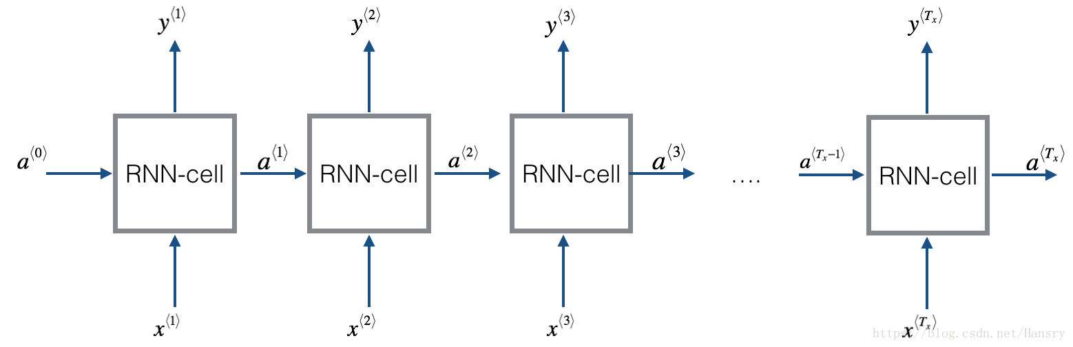
Here’s how you can implement an RNN:

Steps:
1. Implement the calculations needed for one time-step of the RNN. (首先执行1个时间段所需要的计算)
2. Implement a loop over $T_x$ time-steps in order to process all the inputs, one at a time. （执行很多时间步）

Let’s go!

1.1 - RNN cell

A Recurrent neural network can be seen as the repetition of a single cell. You are first going to implement the computations for a single time-step. The following figure describes the operations for a single time-step of an RNN cell.

Figure 2: Basic RNN cell. Takes as input $x^{\langle t \rangle}$ (current input) and $a^{\langle t - 1\rangle}$ (previous hidden state containing information from the past), and outputs $a^{\langle t \rangle}$ which is given to the next RNN cell and also used to predict $y^{\langle t \rangle}$

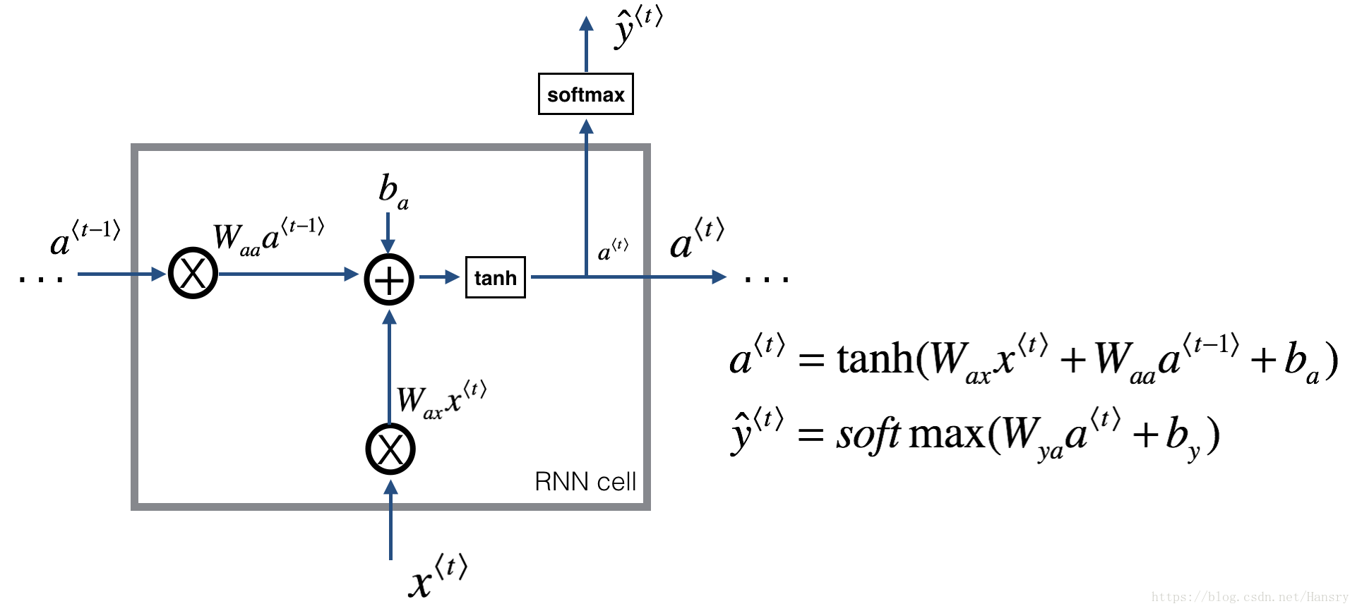
Exercise: Implement the RNN-cell described in Figure (2).

Instructions:
1. Compute the hidden state with tanh activation: $a^{\langle t \rangle} = \tanh(W_{aa} a^{\langle t-1 \rangle} + W_{ax} x^{\langle t \rangle} + b_a)$.
2. Using your new hidden state $a^{\langle t \rangle}$, compute the prediction $\hat{y}^{\langle t \rangle} = softmax(W_{ya} a^{\langle t \rangle} + b_y)$. We provided you a function: softmax.
3. Store $(a^{\langle t \rangle}, a^{\langle t-1 \rangle}, x^{\langle t \rangle}, parameters)$ in cache
4. Return $a^{\langle t \rangle}$ , $y^{\langle t \rangle}$ and cache

We will vectorize over $m$ examples. Thus, $x^{\langle t \rangle}$ will have dimension $(n_x,m)$, and $a^{\langle t \rangle}$ will have dimension $(n_a,m)$.

# GRADED FUNCTION: rnn_cell_forward

def rnn_cell_forward(xt, a_prev, parameters):
    """
    Implements a single forward step of the RNN-cell as described in Figure (2)

    Arguments:
    xt -- your input data at timestep "t", numpy array of shape (n_x, m). 
    a_prev -- Hidden state at timestep "t-1", numpy array of shape (n_a, m)
    parameters -- python dictionary containing:
                        Wax -- Weight matrix multiplying the input, numpy array of shape (n_a, n_x)
                        Waa -- Weight matrix multiplying the hidden state, numpy array of shape (n_a, n_a)
                        Wya -- Weight matrix relating the hidden-state to the output, numpy array of shape (n_y, n_a)
                        ba --  Bias, numpy array of shape (n_a, 1)
                        by -- Bias relating the hidden-state to the output, numpy array of shape (n_y, 1)
    Returns:
    a_next -- next hidden state, of shape (n_a, m)
    yt_pred -- prediction at timestep "t", numpy array of shape (n_y, m)
    cache -- tuple of values needed for the backward pass, contains (a_next, a_prev, xt, parameters)
    """

    # Retrieve parameters from "parameters"
    Wax = parameters["Wax"]
    Waa = parameters["Waa"]
    Wya = parameters["Wya"]
    ba = parameters["ba"]
    by = parameters["by"]

    ### START CODE HERE ### (≈2 lines)
    # compute next activation state using the formula given above
    a_next = np.dot(Wax,xt)+np.dot(Waa,a_prev)+ba
    a_next=  (np.exp(a_next)-np.exp(-a_next))/(np.exp(a_next)+np.exp(-a_next))

    # compute output of the current cell using the formula given above
    yt_pred = softmax(np.dot(Wya,a_next)+by)
    ### END CODE HERE ###

    # store values you need for backward propagation in cache
    cache = (a_next, a_prev, xt, parameters)

    return a_next, yt_pred, cache

Input:

np.random.seed(1)
xt = np.random.randn(3,10)
a_prev = np.random.randn(5,10)
Waa = np.random.randn(5,5)
Wax = np.random.randn(5,3)
Wya = np.random.randn(2,5)
ba = np.random.randn(5,1)
by = np.random.randn(2,1)
parameters = {"Waa": Waa, "Wax": Wax, "Wya": Wya, "ba": ba, "by": by}

a_next, yt_pred, cache = rnn_cell_forward(xt, a_prev, parameters)
print("a_next[4] = ", a_next[4])
print("a_next.shape = ", a_next.shape)
print("yt_pred[1] =", yt_pred[1])
print("yt_pred.shape = ", yt_pred.shape)

Output:

a_next[4] =  [ 0.59584544  0.18141802  0.61311866  0.99808218  0.85016201  0.99980978 -0.18887155  0.99815551  0.6531151   0.82872037]
a_next.shape =  (5, 10)
yt_pred[1] = [ 0.9888161   0.01682021  0.21140899  0.36817467  0.98988387  0.88945212
  0.36920224  0.9966312   0.9982559   0.17746526]
yt_pred.shape =  (2, 10)

1.2 - RNN forward pass

You can see an RNN as the repetition of the cell you’ve just built. If your input sequence of data is carried over 10 time steps, then you will copy the RNN cell 10 times. Each cell takes as input the hidden state from the previous cell ($a^{\langle t-1 \rangle}$) and the current time-step’s input data ($x^{\langle t \rangle}$). It outputs a hidden state ($a^{\langle t \rangle}$) and a prediction ($y^{\langle t \rangle}$) for this time-step.

Figure 3: Basic RNN. The input sequence $x = (x^{\langle 1 \rangle}, x^{\langle 2 \rangle}, ..., x^{\langle T_x \rangle})$ is carried over $T_x$ time steps. The network outputs $y = (y^{\langle 1 \rangle}, y^{\langle 2 \rangle}, ..., y^{\langle T_x \rangle})$.

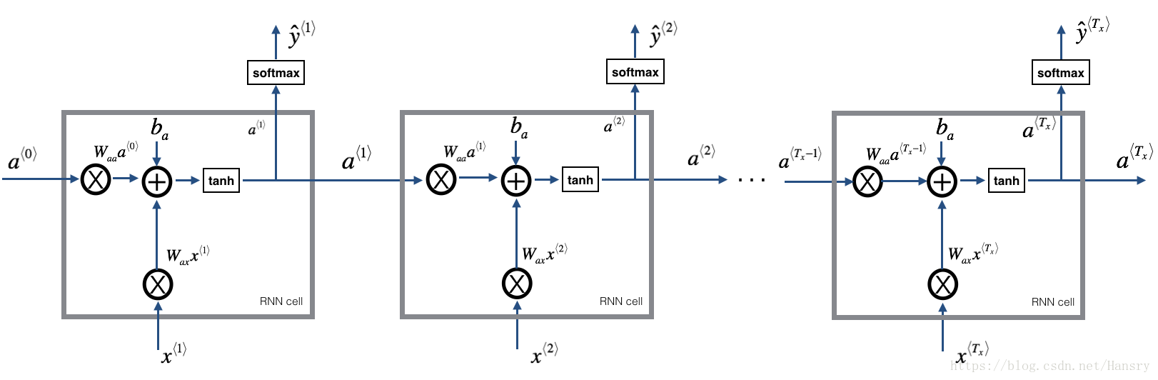
Exercise: Code the forward propagation of the RNN described in Figure (3).

Instructions:
1. Create a vector of zeros ($a$) that will store all the hidden states computed by the RNN.
2. Initialize the “next” hidden state as $a_0$ (initial hidden state).
3. Start looping over each time step, your incremental index is $t$ :
- Update the “next” hidden state and the cache by running rnn_cell_forward
- Store the “next” hidden state in $a$ ($t^{th}$ position)
- Store the prediction in y
- Add the cache to the list of caches
4. Return $a$, $y$ and caches

# GRADED FUNCTION: rnn_forward

def rnn_forward(x, a0, parameters):
    """
    Implement the forward propagation of the recurrent neural network described in Figure (3).

    Arguments:
    x -- Input data for every time-step, of shape (n_x, m, T_x).
    a0 -- Initial hidden state, of shape (n_a, m)
    parameters -- python dictionary containing:
                        Waa -- Weight matrix multiplying the hidden state, numpy array of shape (n_a, n_a)
                        Wax -- Weight matrix multiplying the input, numpy array of shape (n_a, n_x)
                        Wya -- Weight matrix relating the hidden-state to the output, numpy array of shape (n_y, n_a)
                        ba --  Bias numpy array of shape (n_a, 1)
                        by -- Bias relating the hidden-state to the output, numpy array of shape (n_y, 1)

    Returns:
    a -- Hidden states for every time-step, numpy array of shape (n_a, m, T_x)
    y_pred -- Predictions for every time-step, numpy array of shape (n_y, m, T_x)
    caches -- tuple of values needed for the backward pass, contains (list of caches, x)
    """

    # Initialize "caches" which will contain the list of all caches
    caches = []

    # Retrieve dimensions from shapes of x and parameters["Wya"]
    n_x, m, T_x = x.shape
    n_y, n_a = parameters["Wya"].shape

    ### START CODE HERE ###

    # initialize "a" and "y" with zeros (≈2 lines)
    a = np.zeros((n_a,m,x.shape[2]))  
    y_pred = np.zeros((n_y,m,x.shape[2]))

    # Initialize a_next (≈1 line)
    a_next = a0

    # loop over all time-steps
    for t in range(0,x.shape[2]):
        # Update next hidden state, compute the prediction, get the cache (≈1 line)
        a_next, yt_pred, cache = rnn_cell_forward(x[:,:,t], a_next, parameters)  #cache = (a_next, a_prev, xt, parameters)
        # Save the value of the new "next" hidden state in a (≈1 line)
        a[:,:,t] = a_next
        # Save the value of the prediction in y (≈1 line)
        y_pred[:,:,t] = yt_pred
        # Append "cache" to "caches" (≈1 line)
        caches.append(cache)

    ### END CODE HERE ###

    # store values needed for backward propagation in cache
    caches = (caches, x)

    return a, y_pred, caches

Input:

np.random.seed(1)
x = np.random.randn(3,10,4)   #(n_x,m,T_x)
a0 = np.random.randn(5,10)    #(n_a,m)
Waa = np.random.randn(5,5)    #(n_a,n_a)
Wax = np.random.randn(5,3)    #(n_a,n_x)
Wya = np.random.randn(2,5)    #(n_y,n_a)
ba = np.random.randn(5,1)     #(n_a,1)
by = np.random.randn(2,1)     #(n_y,1)
parameters = {"Waa": Waa, "Wax": Wax, "Wya": Wya, "ba": ba, "by": by}

a, y_pred, caches = rnn_forward(x, a0, parameters)
print("a[4][1] = ", a[4][1])
print("a.shape = ", a.shape)
print("y_pred[1][3] =", y_pred[1][3])
print("y_pred.shape = ", y_pred.shape)
print("caches[1][1][3] =", caches[1][1][3])
print("len(caches) = ", len(caches))

Output:

a[4][1] =  [-0.99999375  0.77911235 -0.99861469 -0.99833267]
a.shape =  (5, 10, 4)
y_pred[1][3] = [ 0.79560373  0.86224861  0.11118257  0.81515947]
y_pred.shape =  (2, 10, 4)
caches[1][1][3] = [-1.1425182  -0.34934272 -0.20889423  0.58662319]
len(caches) =  2

2 - Long Short-Term Memory (LSTM) network

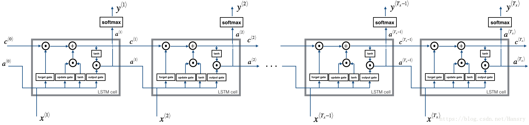
This following figure shows the operations of an LSTM-cell.

Figure 4: LSTM-cell. This tracks and updates a “cell state” or memory variable $c^{\langle t \rangle}$ at every time-step, which can be different from $a^{\langle t \rangle}$.

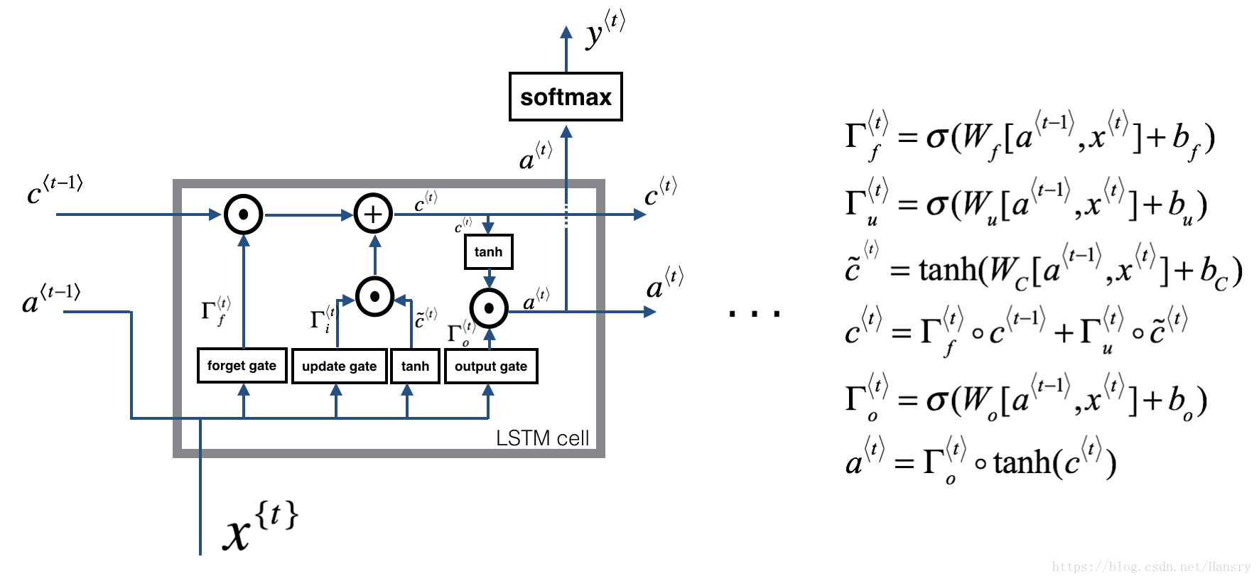
Similar to the RNN example above, you will start by implementing the LSTM cell for a single time-step. Then you can iteratively call it from inside a for-loop to have it process an input with $T_x$ time-steps.

About the gates

- Forget gate

For the sake of this illustration, lets assume we are reading words in a piece of text, and want use an LSTM to keep track of grammatical structures, such as whether the subject is singular or plural. If the subject changes from a singular word to a plural word, we need to find a way to get rid of our previously stored memory value of the singular/plural state. In an LSTM, the forget gate lets us do this

(假如我们现在在处理文件中的一段话，使用LSTM来跟踪语法结构，例如对于一个主语是单数还是复数的，如果主语从单数变成复数，那我们需要忘记之前存储的单复数的状态。在LSTM中，遗忘门就有这个作用。):

$$\Gamma_f^{\langle t \rangle} = \sigma(W_f[a^{\langle t-1 \rangle}, x^{\langle t \rangle}] + b_f)\tag{1}$$

Here, $W_f$ are weights that govern the forget gate’s behavior. We concatenate $[a^{\langle t-1 \rangle}, x^{\langle t \rangle}]$ and multiply by $W_f$. The equation above results in a vector $\Gamma_f^{\langle t \rangle}$ with values between 0 and 1. This forget gate vector will be multiplied element-wise by the previous cell state $c^{\langle t-1 \rangle}$. So if one of the values of $\Gamma_f^{\langle t \rangle}$ is 0 (or close to 0) then it means that the LSTM should remove that piece of information (e.g. the singular subject) in the corresponding component of $c^{\langle t-1 \rangle}$. If one of the values is 1, then it will keep the information.

($W_f$ 是决定遗忘门行为的权重矩阵，将$[a^{\langle t-1 \rangle}, x^{\langle t \rangle}]$ 串联在一起，然后与$W_f$做乘积。这个公式的值域在0和1之间。紧接着用这个遗忘门与$c^{\langle t-1 \rangle}$相乘，如果$\Gamma_f^{\langle t \rangle}$接近于0，那么就相当于选择遗忘$c^{\langle t-1 \rangle}$，如果接近于1，那么就相当于保留$c^{\langle t-1 \rangle}$)

- Update gate

Once we forget that the subject being discussed is singular, we need to find a way to update it to reflect that the new subject is now plural. Here is the formulat for the update gate:

(如果我们选择遗忘上面讨论的主语为单数的状态时，那么我们需要更新其状态为复数，而更新门就是决定是否更新该状态的阈值)

$$\Gamma_u^{\langle t \rangle} = \sigma(W_u[a^{\langle t-1 \rangle}, x^{\{t\}}] + b_u)\tag{2}$$

Similar to the forget gate, here $\Gamma_u^{\langle t \rangle}$ is again a vector of values between 0 and 1. This will be multiplied element-wise with $\tilde{c}^{\langle t \rangle}$, in order to compute $c^{\langle t \rangle}$.

（同样的对于遗忘门，$\Gamma_u^{\langle t \rangle}$的值域也是0到1之间，然后与更新状态 $\tilde{c}^{\langle t \rangle}$相乘）

- Updating the cell

To update the new subject we need to create a new vector of numbers that we can add to our previous cell state. The equation we use is:

（为了更新主语的状态，我们需要创建一个公式，将之前的cell的状态包含进来，公式如下：）

$$\tilde{c}^{\langle t \rangle} = \tanh(W_c[a^{\langle t-1 \rangle}, x^{\langle t \rangle}] + b_c)\tag{3}$$

Finally, the new cell state is:

$$c^{\langle t \rangle} = \Gamma_f^{\langle t \rangle}* c^{\langle t-1 \rangle} + \Gamma_u^{\langle t \rangle} *\tilde{c}^{\langle t \rangle} \tag{4}$$

- Output gate

To decide which outputs we will use, we will use the following two formulas:

$$\Gamma_o^{\langle t \rangle}= \sigma(W_o[a^{\langle t-1 \rangle}, x^{\langle t \rangle}] + b_o)\tag{5}$$
$$a^{\langle t \rangle} = \Gamma_o^{\langle t \rangle}* \tanh(c^{\langle t \rangle})\tag{6}$$

Where in equation 5 you decide what to output using a sigmoid function and in equation 6 you multiply that by the $\tanh$ of the previous state.

2.1 - LSTM cell

Exercise: Implement the LSTM cell described in the Figure (3).

Instructions:
1. Concatenate $a^{\langle t-1 \rangle}$ and $x^{\langle t \rangle}$ in a single matrix: $concat = \begin{bmatrix} a^{\langle t-1 \rangle} \\ x^{\langle t \rangle} \end{bmatrix}$
2. Compute all the formulas 1-6. You can use sigmoid() (provided) and np.tanh().
3. Compute the prediction $y^{\langle t \rangle}$. You can use softmax() (provided).

# GRADED FUNCTION: lstm_cell_forward

def lstm_cell_forward(xt, a_prev, c_prev, parameters):
    """
    Implement a single forward step of the LSTM-cell as described in Figure (4)

    Arguments:
    xt -- your input data at timestep "t", numpy array of shape (n_x, m).
    a_prev -- Hidden state at timestep "t-1", numpy array of shape (n_a, m)
    c_prev -- Memory state at timestep "t-1", numpy array of shape (n_a, m)
    parameters -- python dictionary containing:
                        Wf -- Weight matrix of the forget gate, numpy array of shape (n_a, n_a + n_x)
                        bf -- Bias of the forget gate, numpy array of shape (n_a, 1)
                        Wi -- Weight matrix of the update gate, numpy array of shape (n_a, n_a + n_x)
                        bi -- Bias of the update gate, numpy array of shape (n_a, 1)
                        Wc -- Weight matrix of the first "tanh", numpy array of shape (n_a, n_a + n_x)
                        bc --  Bias of the first "tanh", numpy array of shape (n_a, 1)
                        Wo -- Weight matrix of the output gate, numpy array of shape (n_a, n_a + n_x)
                        bo --  Bias of the output gate, numpy array of shape (n_a, 1)
                        Wy -- Weight matrix relating the hidden-state to the output, numpy array of shape (n_y, n_a)
                        by -- Bias relating the hidden-state to the output, numpy array of shape (n_y, 1)

    Returns:
    a_next -- next hidden state, of shape (n_a, m)
    c_next -- next memory state, of shape (n_a, m)
    yt_pred -- prediction at timestep "t", numpy array of shape (n_y, m)
    cache -- tuple of values needed for the backward pass, contains (a_next, c_next, a_prev, c_prev, xt, parameters)

    Note: ft/it/ot stand for the forget/update/output gates, cct stands for the candidate value (c tilde),
          c stands for the memory value
    """

    # Retrieve parameters from "parameters"
    Wf = parameters["Wf"]
    bf = parameters["bf"]
    Wi = parameters["Wi"]
    bi = parameters["bi"]
    Wc = parameters["Wc"]
    bc = parameters["bc"]
    Wo = parameters["Wo"]
    bo = parameters["bo"]
    Wy = parameters["Wy"]
    by = parameters["by"]

    # Retrieve dimensions from shapes of xt and Wy
    n_x, m = xt.shape
    n_y, n_a = Wy.shape

    ### START CODE HERE ###
    # Concatenate a_prev and xt (≈3 lines)
    concat = np.zeros((a_prev.shape[0]+n_x,m))
    concat[: n_a, :] = a_prev
    concat[n_a :, :] = xt

    # Compute values for ft, it, cct, c_next, ot, a_next using the formulas given figure (4) (≈6 lines)
    ft = sigmoid(np.dot(Wf,concat)+bf)
    it = sigmoid(np.dot(Wi,concat)+bi)
    cct = np.tanh(np.dot(Wc,concat)+bc)
    c_next = ft*c_prev+it*cct
    ot = sigmoid(np.dot(Wo,concat)+bo)
    a_next = ot*np.tanh(c_next)

    # Compute prediction of the LSTM cell (≈1 line)
    yt_pred = softmax(np.dot(Wy,a_next)+by)
    ### END CODE HERE ###

    # store values needed for backward propagation in cache
    cache = (a_next, c_next, a_prev, c_prev, ft, it, cct, ot, xt, parameters)

    return a_next, c_next, yt_pred, cache

Input:

np.random.seed(1)
xt = np.random.randn(3,10)
a_prev = np.random.randn(5,10)
c_prev = np.random.randn(5,10)
Wf = np.random.randn(5, 5+3)
bf = np.random.randn(5,1)
Wi = np.random.randn(5, 5+3)
bi = np.random.randn(5,1)
Wo = np.random.randn(5, 5+3)
bo = np.random.randn(5,1)
Wc = np.random.randn(5, 5+3)
bc = np.random.randn(5,1)
Wy = np.random.randn(2,5)
by = np.random.randn(2,1)

parameters = {"Wf": Wf, "Wi": Wi, "Wo": Wo, "Wc": Wc, "Wy": Wy, "bf": bf, "bi": bi, "bo": bo, "bc": bc, "by": by}

a_next, c_next, yt, cache = lstm_cell_forward(xt, a_prev, c_prev, parameters)
print("a_next[4] = ", a_next[4])
print("a_next.shape = ", c_next.shape)
print("c_next[2] = ", c_next[2])
print("c_next.shape = ", c_next.shape)
print("yt[1] =", yt[1])
print("yt.shape = ", yt.shape)
print("cache[1][3] =", cache[1][3])
print("len(cache) = ", len(cache))

Output:

a_next[4] =  [-0.66408471  0.0036921   0.02088357  0.22834167 -0.85575339  0.00138482
  0.76566531  0.34631421 -0.00215674  0.43827275]
a_next.shape =  (5, 10)
c_next[2] =  [ 0.63267805  1.00570849  0.35504474  0.20690913 -1.64566718  0.11832942
  0.76449811 -0.0981561  -0.74348425 -0.26810932]
c_next.shape =  (5, 10)
yt[1] = [ 0.79913913  0.15986619  0.22412122  0.15606108  0.97057211  0.31146381
  0.00943007  0.12666353  0.39380172  0.07828381]
yt.shape =  (2, 10)
cache[1][3] = [-0.16263996  1.03729328  0.72938082 -0.54101719  0.02752074 -0.30821874
  0.07651101 -1.03752894  1.41219977 -0.37647422]
len(cache) =  10

2.2 - Forward pass for LSTM

Now that you have implemented one step of an LSTM, you can now iterate this over this using a for-loop to process a sequence of $T_x$ inputs.

Figure 4: LSTM over multiple time-steps.

Exercise: Implement lstm_forward() to run an LSTM over $T_x$ time-steps.

Note: $c^{\langle 0 \rangle}$ is initialized with zeros.

def lstm_forward(x, a0, parameters):
    """
    Implement the forward propagation of the recurrent neural network using an LSTM-cell described in Figure (3).

    Arguments:
    x -- Input data for every time-step, of shape (n_x, m, T_x).
    a0 -- Initial hidden state, of shape (n_a, m)
    parameters -- python dictionary containing:
                        Wf -- Weight matrix of the forget gate, numpy array of shape (n_a, n_a + n_x)
                        bf -- Bias of the forget gate, numpy array of shape (n_a, 1)
                        Wi -- Weight matrix of the update gate, numpy array of shape (n_a, n_a + n_x)
                        bi -- Bias of the update gate, numpy array of shape (n_a, 1)
                        Wc -- Weight matrix of the first "tanh", numpy array of shape (n_a, n_a + n_x)
                        bc -- Bias of the first "tanh", numpy array of shape (n_a, 1)
                        Wo -- Weight matrix of the output gate, numpy array of shape (n_a, n_a + n_x)
                        bo -- Bias of the output gate, numpy array of shape (n_a, 1)
                        Wy -- Weight matrix relating the hidden-state to the output, numpy array of shape (n_y, n_a)
                        by -- Bias relating the hidden-state to the output, numpy array of shape (n_y, 1)

    Returns:
    a -- Hidden states for every time-step, numpy array of shape (n_a, m, T_x)
    y -- Predictions for every time-step, numpy array of shape (n_y, m, T_x)
    caches -- tuple of values needed for the backward pass, contains (list of all the caches, x)
    """

    # Initialize "caches", which will track the list of all the caches
    caches = []

    ### START CODE HERE ###
    # Retrieve dimensions from shapes of x and parameters['Wy'] (≈2 lines)
    n_x, m, T_x = x.shape
    n_y, n_a = parameters['Wy'].shape

    # initialize "a", "c" and "y" with zeros (≈3 lines)
    a = np.zeros((n_a,m,T_x))
    c = np.zeros((n_a,m,T_x))
    y = np.zeros((n_y,m,T_x))

    # Initialize a_next and c_next (≈2 lines)
    a_next = a0
    c_next = np.zeros((n_a,m))

    # loop over all time-steps
    for t in range(T_x):
        # Update next hidden state, next memory state, compute the prediction, get the cache (≈1 line)
        a_next, c_next, yt, cache = lstm_cell_forward(x[:,:,t], a_next, c_next, parameters)
        # Save the value of the new "next" hidden state in a (≈1 line)
        a[:,:,t] = a_next
        # Save the value of the prediction in y (≈1 line)
        y[:,:,t] = yt
        # Save the value of the next cell state (≈1 line)
        c[:,:,t]  = c_next
        # Append the cache into caches (≈1 line)
        caches.append(cache)

    ### END CODE HERE ###

    # store values needed for backward propagation in cache
    caches = (caches, x)

    return a, y, c, caches

Input:

np.random.seed(1)
x = np.random.randn(3,10,7)
a0 = np.random.randn(5,10)
Wf = np.random.randn(5, 5+3)
bf = np.random.randn(5,1)
Wi = np.random.randn(5, 5+3)
bi = np.random.randn(5,1)
Wo = np.random.randn(5, 5+3)
bo = np.random.randn(5,1)
Wc = np.random.randn(5, 5+3)
bc = np.random.randn(5,1)
Wy = np.random.randn(2,5)
by = np.random.randn(2,1)

parameters = {"Wf": Wf, "Wi": Wi, "Wo": Wo, "Wc": Wc, "Wy": Wy, "bf": bf, "bi": bi, "bo": bo, "bc": bc, "by": by}

a, y, c, caches = lstm_forward(x, a0, parameters)
print("a[4][3][6] = ", a[4][3][6])
print("a.shape = ", a.shape)
print("y[1][4][3] =", y[1][4][3])
print("y.shape = ", y.shape)
print("caches[1][1[1]] =", caches[1][1][1])
print("c[1][2][1]", c[1][2][1])
print("len(caches) = ", len(caches))

Output:

a[4][3][6] =  0.172117767533
a.shape =  (5, 10, 7)
y[1][4][3] = 0.95087346185
y.shape =  (2, 10, 7)
caches[1][1[1]] = [ 0.82797464  0.23009474  0.76201118 -0.22232814 -0.20075807  0.18656139
  0.41005165]
c[1][2][1] -0.855544916718
len(caches) =  2

3 - Backpropagation in recurrent neural networks (OPTIONAL / UNGRADED)

In modern deep learning frameworks, you only have to implement the forward pass, and the framework takes care of the backward pass, so most deep learning engineers do not need to bother with the details of the backward pass. If however you are an expert in calculus and want to see the details of backprop in RNNs, you can work through this optional portion of the notebook.

（在现在的神经网络款框架中，你只需要执行正向传播，然后这些框架就会接受反向传播，因此大多数神经网络不需要了解反向传播的具体细节。如果你善于计算且想看RNN在反向传播的具体细节，可以继续）

When in an earlier course you implemented a simple (fully connected) neural network, you used backpropagation to compute the derivatives with respect to the cost to update the parameters. Similarly, in recurrent neural networks you can to calculate the derivatives with respect to the cost in order to update the parameters. The backprop equations are quite complicated and we did not derive them in lecture. However, we will briefly present them below.

（在之前的课程中你已经执行了简单的(全连接)神经网络,使用反向传播来计算损失函数的导数来更新参数。相似的，在循环卷积神经网络中，同样可以计算损失函数的导数来更新参数。反向传播的公式相当复杂所以不在该文中推导，只会简单的将他们列出来）

3.1 - Basic RNN backward pass

We will start by computing the backward pass for the basic RNN-cell.

Figure 5: RNN-cell’s backward pass. Just like in a fully-connected neural network, the derivative of the cost function $J$ backpropagates through the RNN by following the chain-rule from calculas. The chain-rule is also used to calculate $(\frac{\partial J}{\partial W_{ax}},\frac{\partial J}{\partial W_{aa}},\frac{\partial J}{\partial b})$ to update the parameters $(W_{ax}, W_{aa}, b_a)$.

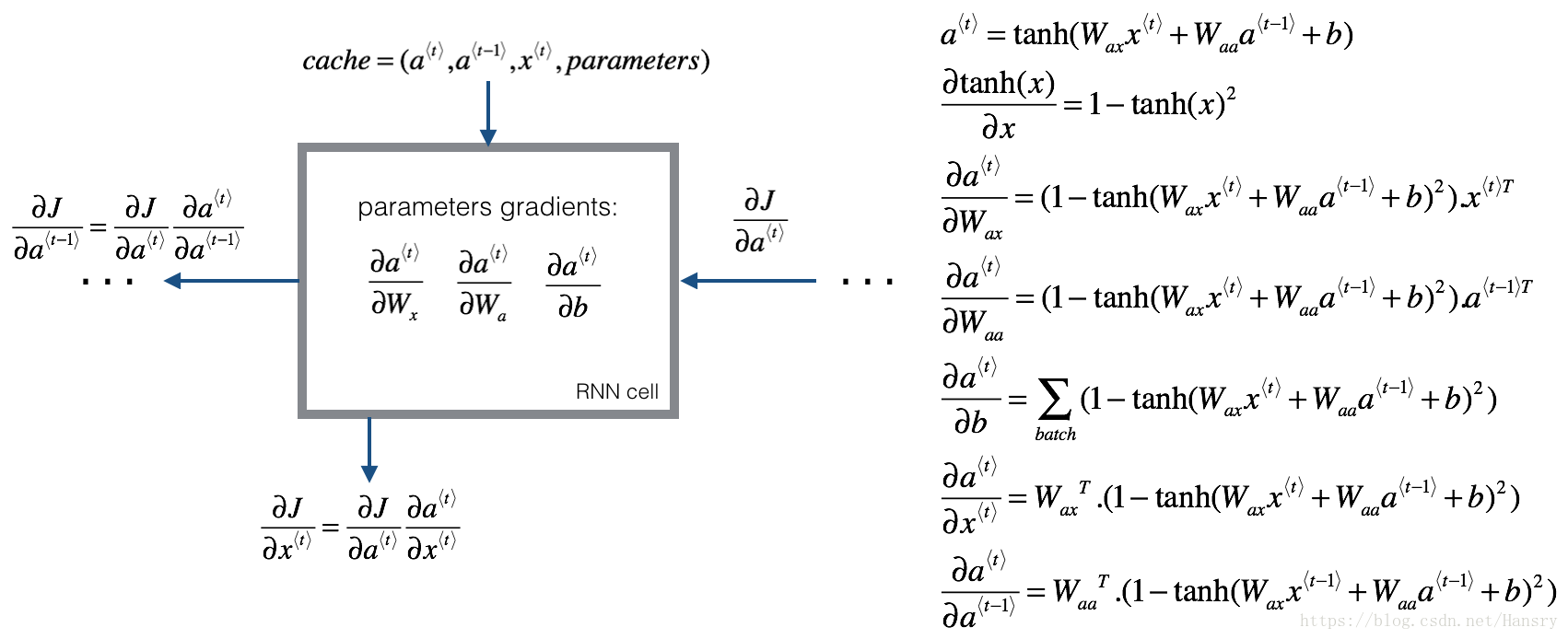
Deriving the one step backward functions:

To compute the rnn_cell_backward you need to compute the following equations. It is a good exercise to derive them by hand.

The derivative of $\tanh$ is $1-\tanh(x)^2$. You can find the complete proof here. Note that: $\text{sech}(x)^2 = 1 - \tanh(x)^2$

Similarly for $\frac{ \partial a^{\langle t \rangle} } {\partial W_{ax}}, \frac{ \partial a^{\langle t \rangle} } {\partial W_{aa}}, \frac{ \partial a^{\langle t \rangle} } {\partial b}$, the derivative of $\tanh(u)$ is $(1-\tanh(u)^2)du$.

The final two equations also follow same rule and are derived using the $\tanh$ derivative. Note that the arrangement is done in a way to get the same dimensions to match.

def rnn_cell_backward(da_next, cache):
    """
    Implements the backward pass for the RNN-cell (single time-step).

    Arguments:
    da_next -- Gradient of loss with respect to next hidden state
    cache -- python dictionary containing useful values (output of rnn_cell_forward())

    Returns:
    gradients -- python dictionary containing:
                        dx -- Gradients of input data, of shape (n_x, m)
                        da_prev -- Gradients of previous hidden state, of shape (n_a, m)
                        dWax -- Gradients of input-to-hidden weights, of shape (n_a, n_x)
                        dWaa -- Gradients of hidden-to-hidden weights, of shape (n_a, n_a)
                        dba -- Gradients of bias vector, of shape (n_a, 1)
    """

    # Retrieve values from cache
    (a_next, a_prev, xt, parameters) = cache

    # Retrieve values from parameters
    Wax = parameters["Wax"]
    Waa = parameters["Waa"]
    Wya = parameters["Wya"]
    ba = parameters["ba"]
    by = parameters["by"]

    ### START CODE HERE ###
    # compute the gradient of tanh with respect to a_next (≈1 line)
    dtanh = (1-a_next**2)*da_next   #(n_a,m)，这里的a_next可能是y^{t}对a的求导，亦可能是对a^{t+1}的求导

    # compute the gradient of the loss with respect to Wax (≈2 lines)
    dxt = np.dot(np.transpose(Wax),dtanh)  # (n_x,m)=(n_a,n_x)^{T}*(n_a,m)
    dWax = np.dot(dtanh,np.transpose(xt))  #(n_a,n_x)

    # compute the gradient with respect to Waa (≈2 lines)
    da_prev = np.dot(np.transpose(Waa),dtanh)  #(n_a,m)
    dWaa = np.dot(dtanh,np.transpose(a_prev))#(na,na)

    # compute the gradient with respect to b (≈1 line)
    dba = np.sum(dtanh,axis=1,keepdims=True)    #(n_a,1),

    ### END CODE HERE ###

    # Store the gradients in a python dictionary
    gradients = {"dxt": dxt, "da_prev": da_prev, "dWax": dWax, "dWaa": dWaa, "dba": dba}

    return gradients

Input:

np.random.seed(1)
xt = np.random.randn(3,10)
a_prev = np.random.randn(5,10)
Wax = np.random.randn(5,3)
Waa = np.random.randn(5,5)
Wya = np.random.randn(2,5)
b = np.random.randn(5,1)
by = np.random.randn(2,1)
parameters = {"Wax": Wax, "Waa": Waa, "Wya": Wya, "ba": ba, "by": by}

a_next, yt, cache = rnn_cell_forward(xt, a_prev, parameters)

da_next = np.random.randn(5,10)
gradients = rnn_cell_backward(da_next, cache)
print("gradients[\"dxt\"][1][2] =", gradients["dxt"][1][2])
print("gradients[\"dxt\"].shape =", gradients["dxt"].shape)
print("gradients[\"da_prev\"][2][3] =", gradients["da_prev"][2][3])
print("gradients[\"da_prev\"].shape =", gradients["da_prev"].shape)
print("gradients[\"dWax\"][3][1] =", gradients["dWax"][3][1])
print("gradients[\"dWax\"].shape =", gradients["dWax"].shape)
print("gradients[\"dWaa\"][1][2] =", gradients["dWaa"][1][2])
print("gradients[\"dWaa\"].shape =", gradients["dWaa"].shape)
print("gradients[\"dba\"][4] =", gradients["dba"][4])
print("gradients[\"dba\"].shape =", gradients["dba"].shape)

Output:

gradients["dxt"][1][2] = -0.460564103059
gradients["dxt"].shape = (3, 10)
gradients["da_prev"][2][3] = 0.0842968653807
gradients["da_prev"].shape = (5, 10)
gradients["dWax"][3][1] = 0.393081873922
gradients["dWax"].shape = (5, 3)
gradients["dWaa"][1][2] = -0.28483955787
gradients["dWaa"].shape = (5, 5)
gradients["dba"][4] = [ 0.80517166]
gradients["dba"].shape = (5, 1)

Backward pass through the RNN

Computing the gradients of the cost with respect to $a^{\langle t \rangle}$ at every time-step $t$ is useful because it is what helps the gradient backpropagate to the previous RNN-cell. To do so, you need to iterate through all the time steps starting at the end, and at each step, you increment the overall $db_a$, $dW_{aa}$, $dW_{ax}$ and you store $dx$.

（计算代价函数的梯度里关于$a^{\lanle t \rangle}$对每一步的$t$是很有用的，因为其在反向传播到达到前一个RNN-cell有重要作用。所以，需要在所有时间段进行迭代，从时间开始到结束，增量式的修改$db_a$, $dW_{aa}$, $dW_{ax}$ 然后存储 $dx$）

Instructions:

Implement the rnn_backward function. Initialize the return variables with zeros first and then loop through all the time steps while calling the rnn_cell_backward at each time timestep, update the other variables accordingly.

def rnn_backward(da, caches):
    """
    Implement the backward pass for a RNN over an entire sequence of input data.

    Arguments:
    da -- Upstream gradients of all hidden states, of shape (n_a, m, T_x)
    caches -- tuple containing information from the forward pass (rnn_forward)

    Returns:
    gradients -- python dictionary containing:
                        dx -- Gradient w.r.t. the input data, numpy-array of shape (n_x, m, T_x)
                        da0 -- Gradient w.r.t the initial hidden state, numpy-array of shape (n_a, m)
                        dWax -- Gradient w.r.t the input's weight matrix, numpy-array of shape (n_a, n_x)
                        dWaa -- Gradient w.r.t the hidden state's weight matrix, numpy-arrayof shape (n_a, n_a)
                        dba -- Gradient w.r.t the bias, of shape (n_a, 1)
    """

    ### START CODE HERE ###

    # Retrieve values from the first cache (t=1) of caches (≈2 lines)
    (caches, x) = caches
    (a1, a0, x1, parameters) = caches[0]  #(a_next, a_prev, xt, parameters) = cache,中间存储的变量

    # Retrieve dimensions from da's and x1's shapes (≈2 lines)
    n_a, m, T_x = da.shape
    n_x, m = x1.shape

    # initialize the gradients with the right sizes (≈6 lines)
    dx = np.zeros((n_x,m,T_x))
    dWax = np.zeros((n_a,n_x))
    dWaa = np.zeros((n_a,n_a))
    dba = np.zeros((n_a,1))
    da0 = np.zeros((n_a,m))
    da_prevt = np.zeros((n_a,m))

    # Loop through all the time steps
    for t in reversed(range(T_x)):
        # Compute gradients at time step t. Choose wisely the "da_next" and the "cache" to use in the backward propagation step. (≈1 line)
        gradients = rnn_cell_backward(da[:,:,t]+da_prevt,caches[t])  
        #这里da[:,:,t]+da_prevt, 一方面来自于y^{t}对a的求导，一方面来自于a^{t+1}对a^{t}的求导
        #其中da[:,:,t]为随机生成的，应该是来自于y^{t}对a的求导

        # Retrieve derivatives from gradients (≈ 1 line)
        dxt, da_prevt, dWaxt, dWaat, dbat = gradients["dxt"], gradients["da_prev"], gradients["dWax"], gradients["dWaa"], gradients["dba"]
        # Increment global derivatives w.r.t parameters by adding their derivative at time-step t (≈4 lines)
        dx[:, :, t] = dxt
        dWax += dWaxt
        dWaa += dWaat
        dba += dbat

    # Set da0 to the gradient of a which has been backpropagated through all time-steps (≈1 line) 
    da0 = da_prevt
    ### END CODE HERE ###

    # Store the gradients in a python dictionary
    gradients = {"dx": dx, "da0": da0, "dWax": dWax, "dWaa": dWaa,"dba": dba}

    return gradients

Input:

np.random.seed(1)
x = np.random.randn(3,10,4)
a0 = np.random.randn(5,10)
Wax = np.random.randn(5,3)
Waa = np.random.randn(5,5)
Wya = np.random.randn(2,5)
ba = np.random.randn(5,1)
by = np.random.randn(2,1)
parameters = {"Wax": Wax, "Waa": Waa, "Wya": Wya, "ba": ba, "by": by}
a, y, caches = rnn_forward(x, a0, parameters)
da = np.random.randn(5, 10, 4)
gradients = rnn_backward(da, caches)

print("gradients[\"dx\"][1][2] =", gradients["dx"][1][2])
print("gradients[\"dx\"].shape =", gradients["dx"].shape)
print("gradients[\"da0\"][2][3] =", gradients["da0"][2][3])
print("gradients[\"da0\"].shape =", gradients["da0"].shape)
print("gradients[\"dWax\"][3][1] =", gradients["dWax"][3][1])
print("gradients[\"dWax\"].shape =", gradients["dWax"].shape)
print("gradients[\"dWaa\"][1][2] =", gradients["dWaa"][1][2])
print("gradients[\"dWaa\"].shape =", gradients["dWaa"].shape)
print("gradients[\"dba\"][4] =", gradients["dba"][4])
print("gradients[\"dba\"].shape =", gradients["dba"].shape)

Output:

gradients["dx"][1][2] = [-2.07101689 -0.59255627  0.02466855  0.01483317]
gradients["dx"].shape = (3, 10, 4)
gradients["da0"][2][3] = -0.314942375127
gradients["da0"].shape = (5, 10)
gradients["dWax"][3][1] = 11.2641044965
gradients["dWax"].shape = (5, 3)
gradients["dWaa"][1][2] = 2.30333312658
gradients["dWaa"].shape = (5, 5)
gradients["dba"][4] = [-0.74747722]
gradients["dba"].shape = (5, 1)

3.2 - LSTM backward pass

3.2.1 One Step backward

The LSTM backward pass is slighltly more complicated than the forward one. We have provided you with all the equations for the LSTM backward pass below. (If you enjoy calculus exercises feel free to try deriving these from scratch yourself.)

3.2.2 gate derivatives

$$d \Gamma_o^{\langle t \rangle} = da_{next}*\tanh(c_{next}) * \Gamma_o^{\langle t \rangle}*(1-\Gamma_o^{\langle t \rangle})\tag{7}$$

$$d\tilde c^{\langle t \rangle} = dc_{next}*\Gamma_u^{\langle t \rangle}+ \Gamma_o^{\langle t \rangle} (1-\tanh(c_{next})^2) * i_t * da_{next} * \tilde c^{\langle t \rangle} * (1-\tanh(\tilde c)^2) \tag{8}$$

$$d\Gamma_u^{\langle t \rangle} = dc_{next}*\tilde c^{\langle t \rangle} + \Gamma_o^{\langle t \rangle} (1-\tanh(c_{next})^2) * \tilde c^{\langle t \rangle} * da_{next}*\Gamma_u^{\langle t \rangle}*(1-\Gamma_u^{\langle t \rangle})\tag{9}$$

$$d\Gamma_f^{\langle t \rangle} = dc_{next}*\tilde c_{prev} + \Gamma_o^{\langle t \rangle} (1-\tanh(c_{next})^2) * c_{prev} * da_{next}*\Gamma_f^{\langle t \rangle}*(1-\Gamma_f^{\langle t \rangle})\tag{10}$$

3.2.3 parameter derivatives

$$dW_f = d\Gamma_f^{\langle t \rangle} * \begin{pmatrix} a_{prev} \\ x_t\end{pmatrix}^T \tag{11}$$
$$dW_u = d\Gamma_u^{\langle t \rangle} * \begin{pmatrix} a_{prev} \\ x_t\end{pmatrix}^T \tag{12}$$
$$dW_c = d\tilde c^{\langle t \rangle} * \begin{pmatrix} a_{prev} \\ x_t\end{pmatrix}^T \tag{13}$$
$$dW_o = d\Gamma_o^{\langle t \rangle} * \begin{pmatrix} a_{prev} \\ x_t\end{pmatrix}^T \tag{14}$$

To calculate $db_f, db_u, db_c, db_o$ you just need to sum across the horizontal (axis= 1) axis on $d\Gamma_f^{\langle t \rangle}, d\Gamma_u^{\langle t \rangle}, d\tilde c^{\langle t \rangle}, d\Gamma_o^{\langle t \rangle}$ respectively. Note that you should have the keep_dims = True option.

Finally, you will compute the derivative with respect to the previous hidden state, previous memory state, and input.

$$da_{prev} = W_f^T*d\Gamma_f^{\langle t \rangle} + W_u^T * d\Gamma_u^{\langle t \rangle}+ W_c^T * d\tilde c^{\langle t \rangle} + W_o^T * d\Gamma_o^{\langle t \rangle} \tag{15}$$
Here, the weights for equations 13 are the first n_a, (i.e. $W_f = W_f[:n_a,:]$ etc…)

$$dc_{prev} = dc_{next}\Gamma_f^{\langle t \rangle} + \Gamma_o^{\langle t \rangle} * (1- \tanh(c_{next})^2)*\Gamma_f^{\langle t \rangle}*da_{next} \tag{16}$$
$$dx^{\langle t \rangle} = W_f^T*d\Gamma_f^{\langle t \rangle} + W_u^T * d\Gamma_u^{\langle t \rangle}+ W_c^T * d\tilde c_t + W_o^T * d\Gamma_o^{\langle t \rangle}\tag{17}$$
where the weights for equation 15 are from n_a to the end, (i.e. $W_f = W_f[n_a:,:]$ etc…)

Exercise: Implement lstm_cell_backward by implementing equations $7-17$ below. Good luck! :)

def lstm_cell_backward(da_next, dc_next, cache):
    """
    Implement the backward pass for the LSTM-cell (single time-step).

    Arguments:
    da_next -- Gradients of next hidden state, of shape (n_a, m)
    dc_next -- Gradients of next cell state, of shape (n_a, m)
    cache -- cache storing information from the forward pass

    Returns:
    gradients -- python dictionary containing:
                        dxt -- Gradient of input data at time-step t, of shape (n_x, m)
                        da_prev -- Gradient w.r.t. the previous hidden state, numpy array of shape (n_a, m)
                        dc_prev -- Gradient w.r.t. the previous memory state, of shape (n_a, m, T_x)
                        dWf -- Gradient w.r.t. the weight matrix of the forget gate, numpy array of shape (n_a, n_a + n_x)
                        dWi -- Gradient w.r.t. the weight matrix of the update gate, numpy array of shape (n_a, n_a + n_x)
                        dWc -- Gradient w.r.t. the weight matrix of the memory gate, numpy array of shape (n_a, n_a + n_x)
                        dWo -- Gradient w.r.t. the weight matrix of the output gate, numpy array of shape (n_a, n_a + n_x)
                        dbf -- Gradient w.r.t. biases of the forget gate, of shape (n_a, 1)
                        dbi -- Gradient w.r.t. biases of the update gate, of shape (n_a, 1)
                        dbc -- Gradient w.r.t. biases of the memory gate, of shape (n_a, 1)
                        dbo -- Gradient w.r.t. biases of the output gate, of shape (n_a, 1)
    """

    # Retrieve information from "cache"
    (a_next, c_next, a_prev, c_prev, ft, it, cct, ot, xt, parameters) = cache

    ### START CODE HERE ###
    # Retrieve dimensions from xt's and a_next's shape (≈2 lines)
    n_x, m = xt.shape
    n_a, m = a_next.shape

    # Compute gates related derivatives, you can find their values can be found by looking carefully at equations (7) to (10) (≈4 lines)
    dot = da_next*np.tanh(c_next)*ot*(1-ot)
    dcct = (dc_next*it+ot*(1-np.square(np.tanh(c_next)))*it*da_next)*(1-np.square(cct))
    dit = (dc_next*cct+ot*(1-np.square(np.tanh(c_next)))*cct*da_next)*it*(1-it)
    dft = (dc_next*c_prev+ot*(1-np.square(np.tanh(c_next)))*c_prev*da_next)*ft*(1-ft) 


    # Compute parameters related derivatives. Use equations (11)-(14) (≈8 lines)
    dWf = np.dot(dft,np.concatenate((a_prev, xt), axis=0).T)
    dWi = np.dot(dit,np.concatenate((a_prev, xt), axis=0).T) 
    dWc = np.dot(dcct,np.concatenate((a_prev, xt), axis=0).T)
    dWo = np.dot(dot,np.concatenate((a_prev, xt), axis=0).T)
    dbf = np.sum(dft,axis=1,keepdims=True)
    dbi = np.sum(dit,axis=1,keepdims=True)
    dbc = np.sum(dcct,axis=1,keepdims=True)
    dbo = np.sum(dot,axis=1,keepdims=True)

    # Compute derivatives w.r.t previous hidden state, previous memory state and input. Use equations (15)-(17). (≈3 lines)
    da_prev = np.dot(parameters['Wf'][:,:n_a].T,dft)+np.dot(parameters['Wi'][:,:n_a].T,dit)+np.dot(parameters['Wc'][:,:n_a].T,dcct)+np.dot(parameters['Wo'][:,:n_a].T,dot) 
    dc_prev = dc_next*ft+ot*(1-np.square(np.tanh(c_next)))*ft*da_next
    dxt = np.dot(parameters['Wf'][:,n_a:].T,dft)+np.dot(parameters['Wi'][:,n_a:].T,dit)+np.dot(parameters['Wc'][:,n_a:].T,dcct)+np.dot(parameters['Wo'][:,n_a:].T,dot) 
    ### END CODE HERE ###

    # Save gradients in dictionary
    gradients = {"dxt": dxt, "da_prev": da_prev, "dc_prev": dc_prev, "dWf": dWf,"dbf": dbf, "dWi": dWi,"dbi": dbi,
                "dWc": dWc,"dbc": dbc, "dWo": dWo,"dbo": dbo}

    return gradients

Input:

np.random.seed(1)
xt = np.random.randn(3,10)
a_prev = np.random.randn(5,10)
c_prev = np.random.randn(5,10)
Wf = np.random.randn(5, 5+3)
bf = np.random.randn(5,1)
Wi = np.random.randn(5, 5+3)
bi = np.random.randn(5,1)
Wo = np.random.randn(5, 5+3)
bo = np.random.randn(5,1)
Wc = np.random.randn(5, 5+3)
bc = np.random.randn(5,1)
Wy = np.random.randn(2,5)
by = np.random.randn(2,1)

parameters = {"Wf": Wf, "Wi": Wi, "Wo": Wo, "Wc": Wc, "Wy": Wy, "bf": bf, "bi": bi, "bo": bo, "bc": bc, "by": by}

a_next, c_next, yt, cache = lstm_cell_forward(xt, a_prev, c_prev, parameters)

da_next = np.random.randn(5,10)
dc_next = np.random.randn(5,10)
gradients = lstm_cell_backward(da_next, dc_next, cache)
print("gradients[\"dxt\"][1][2] =", gradients["dxt"][1][2])
print("gradients[\"dxt\"].shape =", gradients["dxt"].shape)
print("gradients[\"da_prev\"][2][3] =", gradients["da_prev"][2][3])
print("gradients[\"da_prev\"].shape =", gradients["da_prev"].shape)
print("gradients[\"dc_prev\"][2][3] =", gradients["dc_prev"][2][3])
print("gradients[\"dc_prev\"].shape =", gradients["dc_prev"].shape)
print("gradients[\"dWf\"][3][1] =", gradients["dWf"][3][1])
print("gradients[\"dWf\"].shape =", gradients["dWf"].shape)
print("gradients[\"dWi\"][1][2] =", gradients["dWi"][1][2])
print("gradients[\"dWi\"].shape =", gradients["dWi"].shape)
print("gradients[\"dWc\"][3][1] =", gradients["dWc"][3][1])
print("gradients[\"dWc\"].shape =", gradients["dWc"].shape)
print("gradients[\"dWo\"][1][2] =", gradients["dWo"][1][2])
print("gradients[\"dWo\"].shape =", gradients["dWo"].shape)
print("gradients[\"dbf\"][4] =", gradients["dbf"][4])
print("gradients[\"dbf\"].shape =", gradients["dbf"].shape)
print("gradients[\"dbi\"][4] =", gradients["dbi"][4])
print("gradients[\"dbi\"].shape =", gradients["dbi"].shape)
print("gradients[\"dbc\"][4] =", gradients["dbc"][4])
print("gradients[\"dbc\"].shape =", gradients["dbc"].shape)
print("gradients[\"dbo\"][4] =", gradients["dbo"][4])
print("gradients[\"dbo\"].shape =", gradients["dbo"].shape)

Output:

gradients["dxt"][1][2] = 3.23055911511
gradients["dxt"].shape = (3, 10)
gradients["da_prev"][2][3] = -0.0639621419711
gradients["da_prev"].shape = (5, 10)
gradients["dc_prev"][2][3] = 0.797522038797
gradients["dc_prev"].shape = (5, 10)
gradients["dWf"][3][1] = -0.147954838164
gradients["dWf"].shape = (5, 8)
gradients["dWi"][1][2] = 1.05749805523
gradients["dWi"].shape = (5, 8)
gradients["dWc"][3][1] = 2.30456216369
gradients["dWc"].shape = (5, 8)
gradients["dWo"][1][2] = 0.331311595289
gradients["dWo"].shape = (5, 8)
gradients["dbf"][4] = [ 0.18864637]
gradients["dbf"].shape = (5, 1)
gradients["dbi"][4] = [-0.40142491]
gradients["dbi"].shape = (5, 1)
gradients["dbc"][4] = [ 0.25587763]
gradients["dbc"].shape = (5, 1)
gradients["dbo"][4] = [ 0.13893342]
gradients["dbo"].shape = (5, 1)

3.3 Backward pass through the LSTM RNN

This part is very similar to the rnn_backward function you implemented above. You will first create variables of the same dimension as your return variables. You will then iterate over all the time steps starting from the end and call the one step function you implemented for LSTM at each iteration. You will then update the parameters by summing them individually. Finally return a dictionary with the new gradients.

Instructions: Implement the lstm_backward function. Create a for loop starting from $T_x$ and going backward. For each step call lstm_cell_backward and update the your old gradients by adding the new gradients to them. Note that dxt is not updated but is stored.

def lstm_backward(da, caches):

    """
    Implement the backward pass for the RNN with LSTM-cell (over a whole sequence).

    Arguments:
    da -- Gradients w.r.t the hidden states, numpy-array of shape (n_a, m, T_x)
    dc -- Gradients w.r.t the memory states, numpy-array of shape (n_a, m, T_x)
    caches -- cache storing information from the forward pass (lstm_forward)

    Returns:
    gradients -- python dictionary containing:
                        dx -- Gradient of inputs, of shape (n_x, m, T_x)
                        da0 -- Gradient w.r.t. the previous hidden state, numpy array of shape (n_a, m)
                        dWf -- Gradient w.r.t. the weight matrix of the forget gate, numpy array of shape (n_a, n_a + n_x)
                        dWi -- Gradient w.r.t. the weight matrix of the update gate, numpy array of shape (n_a, n_a + n_x)
                        dWc -- Gradient w.r.t. the weight matrix of the memory gate, numpy array of shape (n_a, n_a + n_x)
                        dWo -- Gradient w.r.t. the weight matrix of the save gate, numpy array of shape (n_a, n_a + n_x)
                        dbf -- Gradient w.r.t. biases of the forget gate, of shape (n_a, 1)
                        dbi -- Gradient w.r.t. biases of the update gate, of shape (n_a, 1)
                        dbc -- Gradient w.r.t. biases of the memory gate, of shape (n_a, 1)
                        dbo -- Gradient w.r.t. biases of the save gate, of shape (n_a, 1)
    """

    # Retrieve values from the first cache (t=1) of caches.
    (caches, x) = caches
    (a1, c1, a0, c0, f1, i1, cc1, o1, x1, parameters) = caches[0]

    ### START CODE HERE ###
    # Retrieve dimensions from da's and x1's shapes (≈2 lines)
    n_a, m, T_x = da.shape
    n_x, m = x1.shape

    # initialize the gradients with the right sizes (≈12 lines)
    dx = np.zeros((n_x, m, T_x))
    da0 = np.zeros((n_a, m))  
    da_prevt = np.zeros((n_a, m))  
    dc_prevt = np.zeros((n_a, m))  
    dWf = np.zeros((n_a, n_a + n_x))  
    dWi = np.zeros((n_a, n_a + n_x))  
    dWc = np.zeros((n_a, n_a + n_x))  
    dWo = np.zeros((n_a, n_a + n_x))  
    dbf = np.zeros((n_a, 1))  
    dbi = np.zeros((n_a, 1))  
    dbc = np.zeros((n_a, 1))  
    dbo = np.zeros((n_a, 1)) 

    # loop back over the whole sequence
    for t in reversed(range(T_x)):
        # Compute all gradients using lstm_cell_backward
        gradients = lstm_cell_backward(da[:,:,t]+da_prevt,dc_prevt,caches[t])  
        # Store or add the gradient to the parameters' previous step's gradient
        dx[:, :, t] = gradients['dxt']  
        dWf = dWf+gradients['dWf']  
        dWi = dWi+gradients['dWi']  
        dWc = dWc+gradients['dWc']  
        dWo = dWo+gradients['dWo']  
        dbf = dbf+gradients['dbf']  
        dbi = dbi+gradients['dbi']  
        dbc = dbc+gradients['dbc']  
        dbo = dbo+gradients['dbo'] 
    # Set the first activation's gradient to the backpropagated gradient da_prev.
    da0 = gradients['da_prev']

    ### END CODE HERE ###

    # Store the gradients in a python dictionary
    gradients = {"dx": dx, "da0": da0, "dWf": dWf,"dbf": dbf, "dWi": dWi,"dbi": dbi,
                "dWc": dWc,"dbc": dbc, "dWo": dWo,"dbo": dbo}

    return gradients

Input:

np.random.seed(1)
x = np.random.randn(3,10,7)
a0 = np.random.randn(5,10)
Wf = np.random.randn(5, 5+3)
bf = np.random.randn(5,1)
Wi = np.random.randn(5, 5+3)
bi = np.random.randn(5,1)
Wo = np.random.randn(5, 5+3)
bo = np.random.randn(5,1)
Wc = np.random.randn(5, 5+3)
bc = np.random.randn(5,1)

parameters = {"Wf": Wf, "Wi": Wi, "Wo": Wo, "Wc": Wc, "Wy": Wy, "bf": bf, "bi": bi, "bo": bo, "bc": bc, "by": by}

a, y, c, caches = lstm_forward(x, a0, parameters)

da = np.random.randn(5, 10, 4)
gradients = lstm_backward(da, caches)

print("gradients[\"dx\"][1][2] =", gradients["dx"][1][2])
print("gradients[\"dx\"].shape =", gradients["dx"].shape)
print("gradients[\"da0\"][2][3] =", gradients["da0"][2][3])
print("gradients[\"da0\"].shape =", gradients["da0"].shape)
print("gradients[\"dWf\"][3][1] =", gradients["dWf"][3][1])
print("gradients[\"dWf\"].shape =", gradients["dWf"].shape)
print("gradients[\"dWi\"][1][2] =", gradients["dWi"][1][2])
print("gradients[\"dWi\"].shape =", gradients["dWi"].shape)
print("gradients[\"dWc\"][3][1] =", gradients["dWc"][3][1])
print("gradients[\"dWc\"].shape =", gradients["dWc"].shape)
print("gradients[\"dWo\"][1][2] =", gradients["dWo"][1][2])
print("gradients[\"dWo\"].shape =", gradients["dWo"].shape)
print("gradients[\"dbf\"][4] =", gradients["dbf"][4])
print("gradients[\"dbf\"].shape =", gradients["dbf"].shape)
print("gradients[\"dbi\"][4] =", gradients["dbi"][4])
print("gradients[\"dbi\"].shape =", gradients["dbi"].shape)
print("gradients[\"dbc\"][4] =", gradients["dbc"][4])
print("gradients[\"dbc\"].shape =", gradients["dbc"].shape)
print("gradients[\"dbo\"][4] =", gradients["dbo"][4])
print("gradients[\"dbo\"].shape =", gradients["dbo"].shape)

Output:

gradients["dx"][1][2] = [-0.00173313  0.08287442 -0.30545663 -0.43281115]
gradients["dx"].shape = (3, 10, 4)
gradients["da0"][2][3] = -0.095911501954
gradients["da0"].shape = (5, 10)
gradients["dWf"][3][1] = -0.0698198561274
gradients["dWf"].shape = (5, 8)
gradients["dWi"][1][2] = 0.102371820249
gradients["dWi"].shape = (5, 8)
gradients["dWc"][3][1] = -0.0624983794927
gradients["dWc"].shape = (5, 8)
gradients["dWo"][1][2] = 0.0484389131444
gradients["dWo"].shape = (5, 8)
gradients["dbf"][4] = [-0.0565788]
gradients["dbf"].shape = (5, 1)
gradients["dbi"][4] = [-0.15399065]
gradients["dbi"].shape = (5, 1)
gradients["dbc"][4] = [-0.29691142]
gradients["dbc"].shape = (5, 1)
gradients["dbo"][4] = [-0.29798344]
gradients["dbo"].shape = (5, 1)