文章目录
1. 相关内容
1.1 hist seg:
scipy.signal.find_peaks(x, height=None, threshold=None, distance=None, prominence=None, width=None, wlen=None, rel_height=0.5, plateau_size=None)
scipy.signal.peak_prominences(x, peaks, wlen=None)
    peaks2, properties2 = signal.find_peaks(hist2, distance=5,  prominence=mmax / 20, width=2, plateau_size=[0, 100])
    '''
    distance:两个相邻peak的最小横轴距离
    顶的高度:prominence:突出的程度需满足的条件(顶点一横线,向下平移,直到与更高peak的边交叉。 左右两边取更高的base)
    顶的宽度:width: 一半 prominence位置处的宽度
    plateau_size:允许的平顶的横轴大小范围,
    '''
1.2 pava(parallel Pool Adjacent Violators)
-
What is isotonic regression?
What is nearly-isotonic regression?
很好的两篇博客介绍,isotonic-regression 和 nearly-isotonic-regression,两者的原理如下:前者是强约束,后者是损失函数惩罚
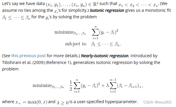
isotonic-regression 是从左向右遍历, 遇到更小的则和当前的块平均,平均后的结果小于更前一个的时候还要再求平均。
两篇博客都提供了动图,是很好的解释。 -
数学解释和实现介绍了相关数学原理。
-
scipy中的isotonic regression 函数 如何用python调用
-
中文解释和博客:
https://github.com/endymecy/spark-ml-source-analysis/blob/master/%E5%88%86%E7%B1%BB%E5%92%8C%E5%9B%9E%E5%BD%92/%E4%BF%9D%E5%BA%8F%E5%9B%9E%E5%BD%92/isotonic-regression.md
https://cloud.tencent.com/developer/article/1815613
1.3 TPS(thin plate splines)
[薄板样条插值(Thin Plate Spline)]https://zhuanlan.zhihu.com/p/227857813
介绍了数学原理推导
数值方法——薄板样条插值(Thin-Plate Spline)
[外链图片转存失败,源站可能有防盗链机制,建议将图片保存下来直接上传(img-O6SQm7iS-1681722986585)(2023-04-06-16-48-11.png)]
薄板样条函数(Thin plate splines)的讨论与分析
2d tps的数学原理概述,总的来说就是tps得到的结果会使整个曲面的弯曲能量最小:
薄板样条插值(Thin plate splines)的实现与使用 pytorch 的实现,opencv的使用
opencv使用:
def tps_cv2(source, target, img):
    """
    使用cv2自带的tps处理
    """
    tps = cv2.createThinPlateSplineShapeTransformer()

    source_cv2 = source.reshape(1, -1, 2)
    target_cv2 = target.reshape(1, -1, 2)

    matches = list()
    for i in range(0, len(source_cv2[0])):
        matches.append(cv2.DMatch(i,i,0))

    tps.estimateTransformation(target_cv2, source_cv2, matches)
    new_img_cv2 = tps.warpImage(img)

    return new_img_cv2
pytorch实现:
def tps_torch(source, target, img, DEVICE):
    """
    使用pyotrch实现的tps处理
    """
    ten_img = ToTensor()(img).to(DEVICE)
    h, w = ten_img.shape[1], ten_img.shape[2]

    ten_source = norm(source, w, h)
    ten_target = norm(target, w, h)
    tpsb = TPS(size=(h, w), device=DEVICE)

    warped_grid = tpsb(ten_target[None, ...], ten_source[None, ...])    #[bs, h, w, 2](相对)   根据source、target得到的仿射函数,处理图片
    ten_wrp = torch.grid_sampler_2d(ten_img[None, ...], warped_grid, 0, 0, False)
    new_img_torch = np.array(ToPILImage()(ten_wrp[0].cpu()))

    return new_img_torch
3D tps:This is a Python reimplementation of the MATLAB version by Yang Yang
Thin Plate Spline
2. 基于optimal transpoet的 color transfer
1. 相关文章
- Adaptive Color Transfer With Relaxed Optimal Transport
- REGULARIZED DISCRETE OPTIMAL TRANSPORT
- Optimal Transportation for Example-Guided Color Transfer
2. REGULARIZED DISCRETE OPTIMAL TRANSPORT 论文 损失
损失目标是:
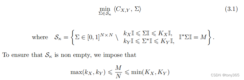
有点类似Partial optimal transport的损失,不过Partial optimal transport只包含了Kx, Ky的约束,未包含 kx, ky
此外Partial optimal transport 有ot.partial.entropic_partial_wasserstein 熵约束。
该论文提出了基于图的梯度约束。
具体如下:
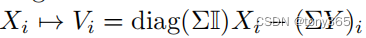
首先 假设我们想要的映射矩阵是 T(下面公式种的求和符号):X 转换为 Y
Xi的的转换为

为了凸优化:
然后构建一个图, Xi最近的 K 个邻居链接为边。
每条边的weight:
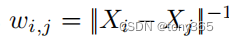
则 T在 Xi上的约束为:

所有边的约束:
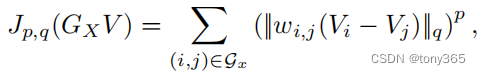
最终的损失函数:

3. REGULARIZED DISCRETE OPTIMAL TRANSPORT 论文
注意 transfer seg的方法
和 transfer pixel的方法
本文中的方法就是pot lib中 transform
其次 找到对应关系之后,可以用多项式拟合或者TPS来拟合。
Optimal Transportation for Example-Guided Color Transfer就是用tps拟合的