目录
1.选取数据
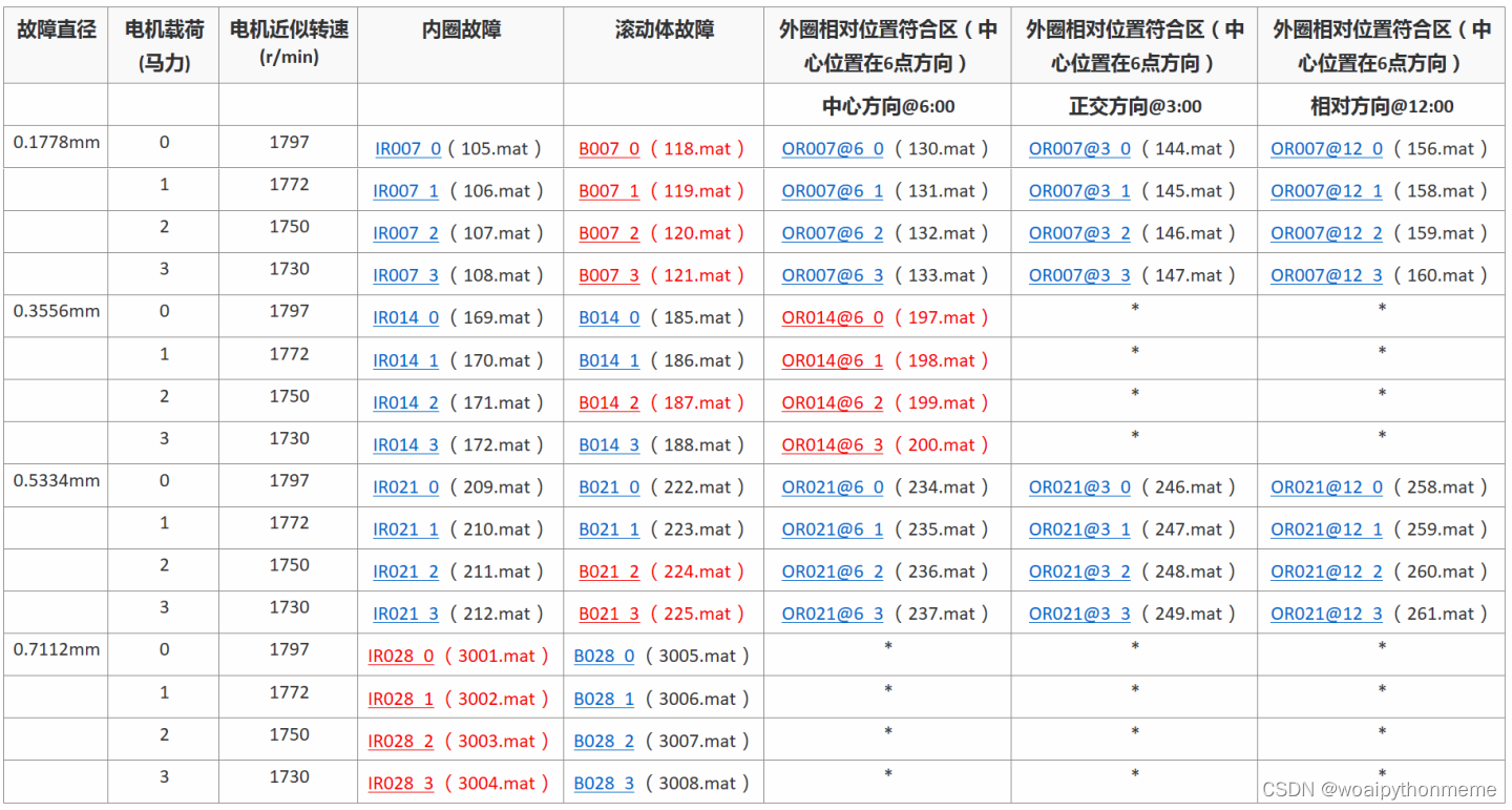
选取1797转速下的内圈故障数据,也就是105.mat,数据集可以在官网下载。下载数据文件|凯斯工程学院 |凯斯西储大学 (case.edu)![]() https://engineering.case.edu/bearingdatacenter/download-data-file
https://engineering.case.edu/bearingdatacenter/download-data-file
2.VMD函数-matlab代码
VMD函数的matlab代码实现,该代码作为函数实现,无需修改,直接使用即可。
function [u, u_hat, omega] = VMD(signal, alpha, tau, K, DC, init, tol)
% Variational Mode Decomposition

% Input and Parameters:
% ---------------------
% signal  - the time domain signal (1D) to be decomposed
% alpha   - the balancing parameter of the data-fidelity constraint 惩罚因子
% tau     - time-step of the dual ascent ( pick 0 for noise-slack )
% K       - the number of modes to be recovered 模态分量
% DC      - true if the first mode is put and kept at DC (0-freq)
% init    - 0 = all omegas start at 0
%                    1 = all omegas start uniformly distributed
%                    2 = all omegas initialized randomly
% tol     - tolerance of convergence criterion; typically around 1e-6
%
% Output:
% -------
% u       - the collection of decomposed modes
% u_hat   - spectra of the modes
% omega   - estimated mode center-frequencies


%---------- Preparations
% Period and sampling frequency of input signal
save_T = length(signal);
fs = 1/save_T;

% extend the signal by mirroring
T = save_T;
f_mirror(1:T/2) = signal(T/2:-1:1);
f_mirror(T/2+1:3*T/2) = signal;
f_mirror(3*T/2+1:2*T) = signal(T:-1:T/2+1);
f = f_mirror;

% Time Domain 0 to T (of mirrored signal)
T = length(f);
t = (1:T)/T;

% Spectral Domain discretization
freqs = t-0.5-1/T;

% Maximum number of iterations (if not converged yet, then it won't anyway)
N = 500;

% For future generalizations: individual alpha for each mode
Alpha = alpha*ones(1,K);

% Construct and center f_hat
f_hat = fftshift((fft(f)));
f_hat_plus = f_hat;
f_hat_plus(1:T/2) = 0;

% matrix keeping track of every iterant // could be discarded for mem
u_hat_plus = zeros(N, length(freqs), K);

% Initialization of omega_k
omega_plus = zeros(N, K);
switch init
    case 1
        for i = 1:K
            omega_plus(1,i) = (0.5/K)*(i-1);
        end
    case 2
        omega_plus(1,:) = sort(exp(log(fs) + (log(0.5)-log(fs))*rand(1,K)));
    otherwise
        omega_plus(1,:) = 0;
end

% if DC mode imposed, set its omega to 0
if DC
    omega_plus(1,1) = 0;
end

% start with empty dual variables
lambda_hat = zeros(N, length(freqs));

% other inits
uDiff = tol+eps; % update step
n = 1; % loop counter
sum_uk = 0; % accumulator


% ----------- Main loop for iterative updates


while ( uDiff > tol &&  n < N ) % not converged and below iterations limit

    % update first mode accumulator
    k = 1;
    sum_uk = u_hat_plus(n,:,K) + sum_uk - u_hat_plus(n,:,1);

    % update spectrum of first mode through Wiener filter of residuals
    u_hat_plus(n+1,:,k) = (f_hat_plus - sum_uk - lambda_hat(n,:)/2)./(1+Alpha(1,k)*(freqs - omega_plus(n,k)).^2);

    % update first omega if not held at 0
    if ~DC
        omega_plus(n+1,k) = (freqs(T/2+1:T)*(abs(u_hat_plus(n+1, T/2+1:T, k)).^2)')/sum(abs(u_hat_plus(n+1,T/2+1:T,k)).^2);
    end

    % update of any other mode
    for k=2:K

        % accumulator
        sum_uk = u_hat_plus(n+1,:,k-1) + sum_uk - u_hat_plus(n,:,k);

        % mode spectrum
        u_hat_plus(n+1,:,k) = (f_hat_plus - sum_uk - lambda_hat(n,:)/2)./(1+Alpha(1,k)*(freqs - omega_plus(n,k)).^2);

        % center frequencies
        omega_plus(n+1,k) = (freqs(T/2+1:T)*(abs(u_hat_plus(n+1, T/2+1:T, k)).^2)')/sum(abs(u_hat_plus(n+1,T/2+1:T,k)).^2);

    end

    % Dual ascent
    lambda_hat(n+1,:) = lambda_hat(n,:) + tau*(sum(u_hat_plus(n+1,:,:),3) - f_hat_plus);

    % loop counter
    n = n+1;

    % converged yet?
    uDiff = eps;
    for i=1:K
        uDiff = uDiff + 1/T*(u_hat_plus(n,:,i)-u_hat_plus(n-1,:,i))*conj((u_hat_plus(n,:,i)-u_hat_plus(n-1,:,i)))';
    end
    uDiff = abs(uDiff);

end


%------ Postprocessing and cleanup


% discard empty space if converged early
N = min(N,n);
omega = omega_plus(1:N,:);

% Signal reconstruction
u_hat = zeros(T, K);
u_hat((T/2+1):T,:) = squeeze(u_hat_plus(N,(T/2+1):T,:));
u_hat((T/2+1):-1:2,:) = squeeze(conj(u_hat_plus(N,(T/2+1):T,:)));
u_hat(1,:) = conj(u_hat(end,:));

u = zeros(K,length(t));

for k = 1:K
    u(k,:)=real(ifft(ifftshift(u_hat(:,k))));
end

% remove mirror part
u = u(:,T/4+1:3*T/4);

% recompute spectrum
clear u_hat;
for k = 1:K
    u_hat(:,k)=fftshift(fft(u(k,:)))';
end

end
3.采用matlab脚本导入数据并做VMD分解
该段代码将内圈故障数据导入,并进行了VMD分解。其中得到的u即为分解出来的IMF分量。
clc
clear
fs=12000;%采样频率
Ts=1/fs;%采样周期
L=1500;%采样点数
t=(0:L-1)*Ts;%时间序列
STA=1; %采样起始位置
%----------------导入内圈故障的数据-----------------------------------------
load 105.mat
X = X105_DE_time(1:L)'; %这里可以选取DE(驱动端加速度)、FE(风扇端加速度)、BA(基座加速度),直接更改变量名,挑选一种即可。

%--------- some sample parameters forVMD:对于VMD样品参数进行设置---------------
alpha = 2500;       % moderate bandwidth constraint:适度的带宽约束/惩罚因子
tau = 0;          % noise-tolerance (no strict fidelity enforcement):噪声容限(没有严格的保真度执行)
K = 8;              % modes:分解的模态数,可以自行设置,这里以8为例。
DC = 0;             % no DC part imposed:无直流部分
init = 1;           % initialize omegas uniformly  :omegas的均匀初始化
tol = 1e-7;
%--------------- Run actual VMD code:数据进行vmd分解---------------------------
[u, u_hat, omega] = VMD(X, alpha, tau, K, DC, init, tol); %其中u为分解得到的IMF分量
4. VMD分解图
该段代码用于作图,图片可以参考下面的结果展示。
figure(1);
imfn=u;
n=size(imfn,1);
subplot(n+1,1,1);
plot(t,X); %故障信号
ylabel('原始信号','fontsize',12,'fontname','宋体');

for n1=1:n
    subplot(n+1,1,n1+1);
    plot(t,u(n1,:));%输出IMF分量,a(:,n)则表示矩阵a的第n列元素,u(n1,:)表示矩阵u的n1行元素
    ylabel(['IMF' int2str(n1)]);%int2str(i)是将数值i四舍五入后转变成字符,y轴命名
end
 xlabel('时间\itt/s','fontsize',12,'fontname','宋体');
5.计算中心频率
 %----------------------计算中心频率确定分解个数K-----------------------------
average=mean(omega);  %对omega求平均值,即为中心频率。
中心频率可以用来确定模态分量K的个数,average即为计算得出的中心频率。因为是要确定分解层数,将K设置不同的值,例如1-9,比较最后一个分量的频率。可以确定K值的依据为:一旦出现相似频率,此时的K值被确定为最佳K值。
6.画包络线
该段代码用来画包络线,图形参考下面的结果展示。
figure(2)
for i = 1:K
	Hy(i,:)= abs(hilbert(u(i,:)));
    subplot(K,1,i);
    plot(t,u(i,:),'k',t,Hy(i,:),'r');
     xlabel('样点'); ylabel('幅值')
     grid; legend('信号','包络');
end
title('信号和包络');
set(gcf,'color','w');
7. 画包络谱
该段代码用来画包络谱,图形参考下面的结果展示。
画包络谱的时候,切记要将 “nfft” 设置为采样点数的一半。
% 画包络谱
figure('Name','包络谱','Color','white');
nfft=fix(L/2);
for i = 1:K
    p=abs(fft(Hy(i,:))); %并fft,得到p,就是包络线的fft---包络谱
    p = p/length(p)*2;
    p = p(1: fix(length(p)/2));
    subplot(K,1,i);
    plot((0:nfft-1)/nfft*fs/2,p)   %绘制包络谱
    %xlim([0 600]) %展示包络谱低频段,这句代码可以自己根据情况选择是否注释
     if i ==1
    title('包络谱'); xlabel('频率'); ylabel('幅值')
     else
        xlabel('频率'); ylabel('幅值')
     end
end
set(gcf,'color','w');
8. 计算峭度值
%% 计算峭度值
for i=1:K
  a(i)=kurtosis(imfn(i,:));%峭度
  disp(['IMF',num2str(i),'的峭度值为:',num2str(a(i))])
end
figure
b = bar(a,0.3);
xlabel('模态函数'); ylabel('峭度值')
set(gca,'xtick',1:1:K);
set(gca,'xticklabel',{'IMF1','IMF2','IMF3','IMF4','IMF5','IMF6','IMF7','IMF8'});
xtips1 = b.XEndPoints;
ytips1 = b.YEndPoints; %获取Bar对象的XEndPoints和YEndPoints属性
labels1 = string(b.YData); %获取条形末端坐标
text(xtips1, ytips1, labels1, 'HorizontalAlignment', 'center', 'VerticalAlignment', 'bottom');
%指定垂直、水平对其,让值显示在条形末端居中
9.计算能量和能量熵
%% 能量熵
for i=1:K
   Eimf(i) = sum(imfn(i,:).^2,2);
end
disp(['IMF分量的能量'])
disp(Eimf(1:K))
% 能量熵
E = sum(Eimf);
for j = 1:K
    p(j) = Eimf(j)/E;
    HE(j)=-sum(p(j).*log(p(j)));
end
disp('EMD能量熵=%.4f');
disp(HE(1:K));
10.近似熵代码
近似熵函数,直接复制粘贴,不用改函数。
%近似熵函数的代码
function ApEn = kApproximateEntropy(data, dim, r)
% 计算近似熵(ApEn)
% data - 待分析数据,需要是一维数据
% dim - 模式维度
% r- 阈值大小,一船选择r=0.1-0.25,
data = data(:); %强制转化数据为列方向
N = length(data);%获取数据长度
result = zeros(1,2);%初始化参数
for j = 1:2
m = dim+j-1;
C = zeros(1,N-m+1);%C值初始化,
dataMat = zeros (m, N-m+1);%初始化
for i = 1:m
dataMat(i,:) = data(i:N-m+i); %
end
% counting similar patterns using distance calculation
for i = 1:N-m+1
tempMat = abs(dataMat - repmat (dataMat(:,i),1,N-m+1));
boolMat = any((tempMat>r),1);
C(i)=sum(~boolMat)/(N-m+1);
end
phi(j) = sum(log(C))/(N-m+1);
end
ApEn = phi(1)-phi(2);
end
近似熵调用:对每个IMF分量计算近似熵
for i1=1:K
    imf0=imfn(i1,:);%
    x=imf0';
    ApEnx = kApproximateEntropy(x, 2, 0.15);    %多尺度熵计算
    ApEn(1,i1)= ApEnx;
    disp(['IMF',num2str(i1),'的近似熵为:',num2str(ApEn(1,i1))])
end
11.包络熵
包络熵调用:对每个IMF分量计算包络熵
for i = 1:K
xx= abs(hilbert(u(i,:))); %最小包络熵计算公式!
xxx = xx/sum(xx);
ssum=0;
for ii = 1:size(xxx,2)
bb = xxx(1,ii)*log(xxx(1,ii));
ssum=ssum+bb;
end
Enen(i,:) = -ssum;%每个IMF分量的包络熵
disp(['IMF',num2str(i),'的包络熵为:',num2str(Enen(i,:))])
end
ff = min(Enen);%求取局部最小包络熵,一般用智能优化算法优化VMD,最为最小适应度函数使用
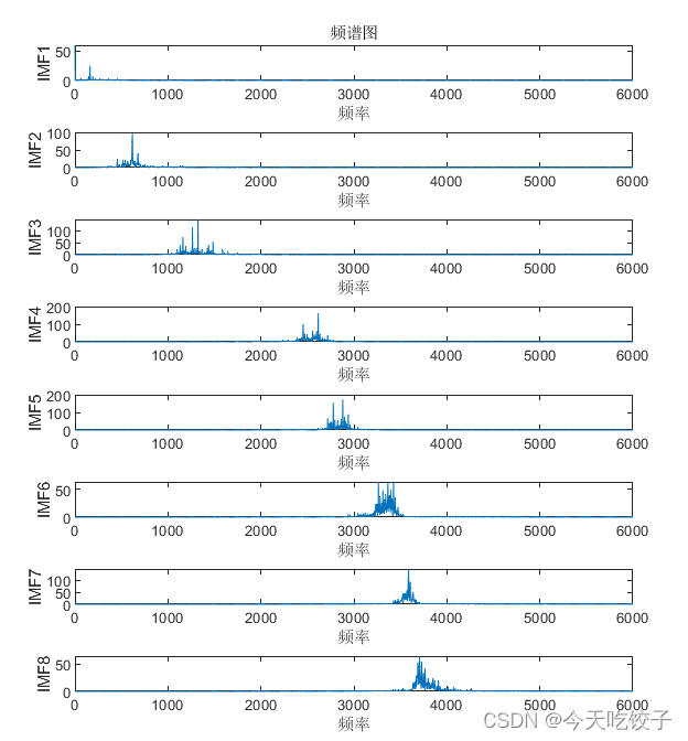
disp(['局部最小包络熵为:',num2str(ff)])12.频谱图
figure('Name','频谱图','Color','white');
for i = 1:K
    p=abs(fft(u(i,:))); %并fft,得到p,就是包络线的fft---包络谱
    subplot(K,1,i);
    plot((0:L-1)*fs/L,p)   %绘制包络谱
    xlim([0 fs/2]) %展示包络谱低频段,这句代码可以自己根据情况选择是否注释
     if i ==1
    title('频谱图'); xlabel('频率'); ylabel(['IMF' int2str(i)]);%int2str(i)是将数值i四舍五入后转变成字符,y轴命名
     else
        xlabel('频率');  ylabel(['IMF' int2str(i)]);%int2str(i)是将数值i四舍五入后转变成字符,y轴命名
     end
end
set(gcf,'color','w');
13.结果展示
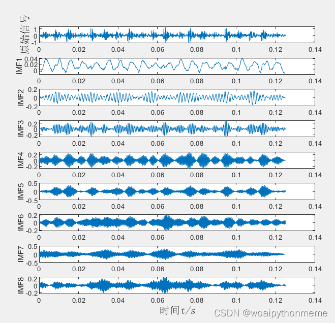 VMD分解图
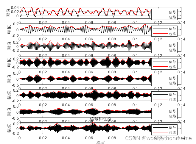
包络线图
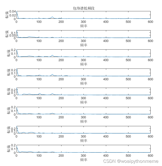
包络熵低频段
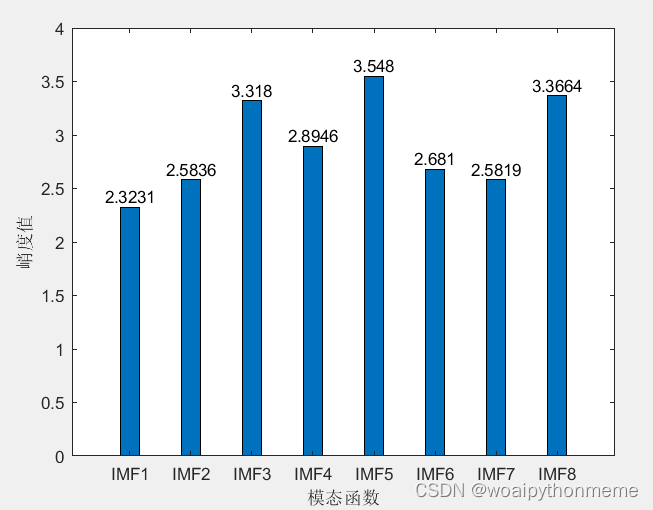 峭度值
峭度值
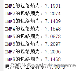
包络熵计算
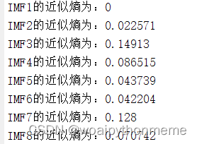
近似熵
13.智能算法优化VMD参数
智能算法优化VMD参数将在下一篇文章介绍!敬请关注谢谢!
(2条消息) 麻雀算法SSA,优化VMD,适应度函数为最小包络熵,包含MATLAB源代码,直接复制粘贴!_今天吃饺子的博客-CSDN博客