《MATLAB 神经网络43个案例分析》：第42章 并行运算与神经网络——基于CPU/GPU的并行神经网络运算

1. 前言

《MATLAB 神经网络43个案例分析》是MATLAB技术论坛（www.matlabsky.com）策划，由王小川老师主导，2013年北京航空航天大学出版社出版的关于MATLAB为工具的一本MATLAB实例教学书籍，是在《MATLAB神经网络30个案例分析》的基础上修改、补充而成的，秉承着“理论讲解—案例分析—应用扩展”这一特色，帮助读者更加直观、生动地学习神经网络。

《MATLAB神经网络43个案例分析》共有43章，内容涵盖常见的神经网络（BP、RBF、SOM、Hopfield、Elman、LVQ、Kohonen、GRNN、NARX等）以及相关智能算法（SVM、决策树、随机森林、极限学习机等）。同时，部分章节也涉及了常见的优化算法（遗传算法、蚁群算法等）与神经网络的结合问题。此外，《MATLAB神经网络43个案例分析》还介绍了MATLAB R2012b中神经网络工具箱的新增功能与特性，如神经网络并行计算、定制神经网络、神经网络高效编程等。

近年来随着人工智能研究的兴起，神经网络这个相关方向也迎来了又一阵研究热潮，由于其在信号处理领域中的不俗表现，神经网络方法也在不断深入应用到语音和图像方向的各种应用当中，本文结合书中案例，对其进行仿真实现，也算是进行一次重新学习，希望可以温故知新，加强并提升自己对神经网络这一方法在各领域中应用的理解与实践。自己正好在多抓鱼上入手了这本书，下面开始进行仿真示例，主要以介绍各章节中源码应用示例为主，本文主要基于MATLAB2018a(64位，MATLAB2015b未安装并行处理工具箱)平台仿真实现，这是本书第四十二章并行运算与神经网络实例，话不多说，开始！

2. MATLAB 仿真示例一

打开MATLAB，点击“主页”，点击“打开”，找到示例文件

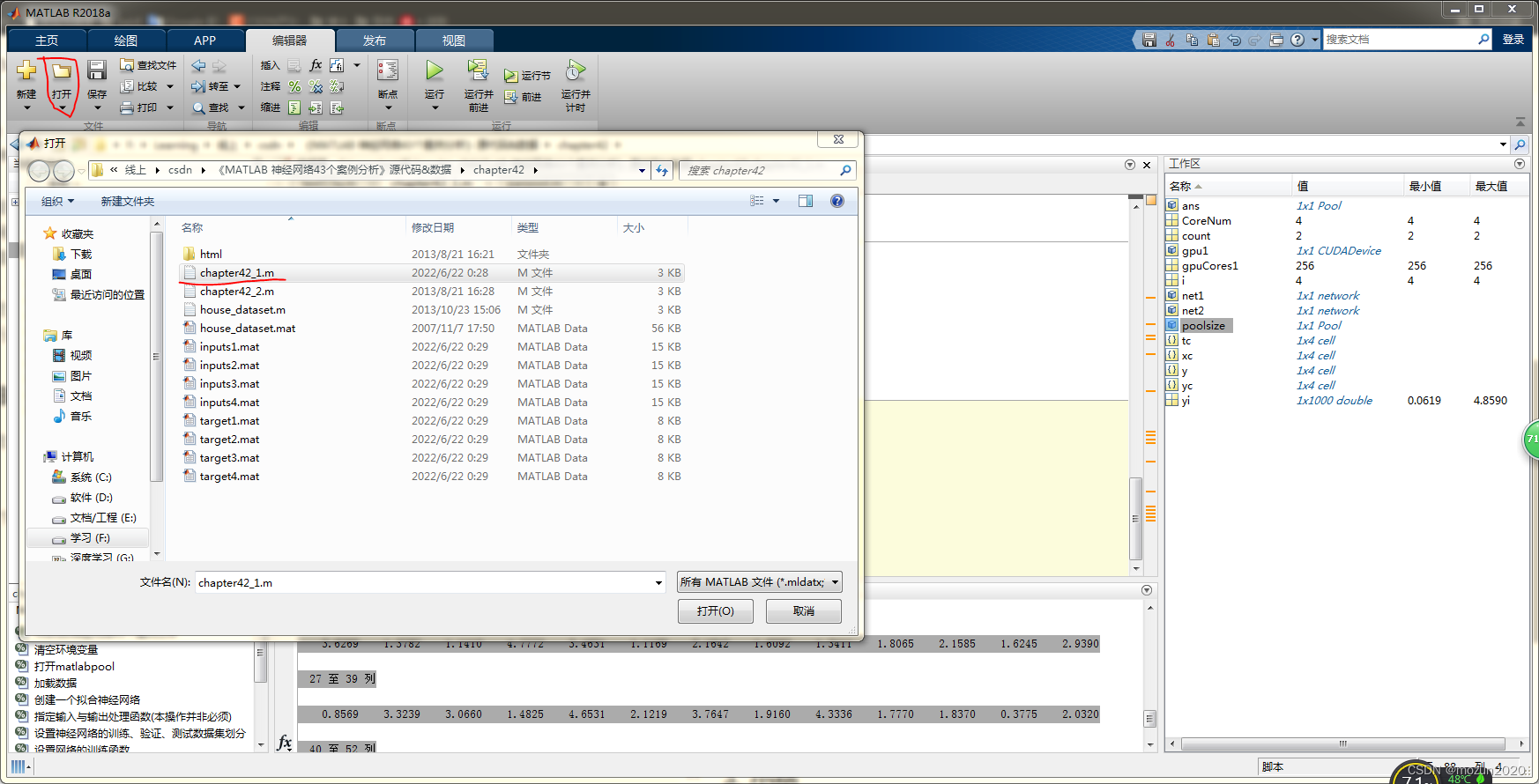
选中chapter42_1.m，点击“打开”

chapter42_1.m源码如下：

%%%%%%%%%%%%%%%%%%%%%%%%%%%%%%%%%%%%%%%%%%%%%%%%%%%%
%功能：并行运算与神经网络-基于CPU/GPU的并行神经网络运算
%环境：Win7，Matlab2015b
%Modi: C.S
%时间：2022-06-21
%%%%%%%%%%%%%%%%%%%%%%%%%%%%%%%%%%%%%%%%%%%%%%%%%%%%


%% Matlab神经网络43个案例分析

% 并行运算与神经网络-基于CPU/GPU的并行神经网络运算
% by 王小川(@王小川_matlab)
% http://www.matlabsky.com
% Email:sina363@163.com
% http://weibo.com/hgsz2003
% 本代码为示例代码脚本，建议不要整体运行，运行时注意备注提示。
close all;
clear all 
clc

tic
%% CPU并行
%% 标准单线程的神经网络训练与仿真过程
[x,t]=house_dataset;
net1=feedforwardnet(10);
net2=train(net1,x,t);
y=sim(net2,x);

%% 打开MATLAB workers
% matlabpool open

% 检查worker数量
delete(gcp('nocreate'))
poolsize=parpool(2)

%% 设置train与sim函数中的参数“Useparallel”为“yes”。
net2=train(net1,x,t,'Useparallel','yes')
y=sim(net2,x,'Useparallel','yes');

%% 使用“showResources”选项证实神经网络运算确实在各个worker上运行。
net2=train(net1,x,t,'useParallel','yes','showResources','yes');
y=sim(net2,x,'useParallel','yes','showResources','yes');

%% 将一个数据集进行随机划分，同时保存到不同的文件
CoreNum=2; %设定机器CPU核心数量
if isempty(gcp('nocreate'))
    parpool(CoreNum);
end
for i=1:2
x=rand(2,1000);
save(['inputs' num2str(i)],'x')
t=x(1,:).*x(2,:)+2*(x(1,:)+x(2,:)) ;
save(['target' num2str(i)],'t');
clear x t
end

%% 实现并行运算加载数据集　
CoreNum=2; %设定机器CPU核心数量
if isempty(gcp('nocreate'))
    parpool(CoreNum);
end
for i=1:2
    data=load(['inputs' num2str(i)],'x');
    xc{
    
    i}=data.x;
    data=load(['target' num2str(i)],'t');
    tc{
    
    i}=data.t;
    clear data
end
net2=configure(net2,xc{
    
    1},tc{
    
    1});
net2=train(net2,xc,tc);
yc=sim(net2,xc);

%% 得到各个worker返回的Composite结果
CoreNum=2; %设定机器CPU核心数量
if isempty(gcp('nocreate'))
    parpool(CoreNum);
end
for i=1:2
    yi=yc{
    
    i};
end

%% GPU并行
count=gpuDeviceCount
gpu1=gpuDevice(1)
gpuCores1=gpu1.MultiprocessorCount*gpu1.SIMDWidth
net2=train(net1,xc,tc,'useGPU','yes')
y=sim(net2,xc,'useGPU','yes')
net1.trainFcn='trainscg';
net2=train(net1,xc,tc,'useGPU','yes','showResources','yes');
y=sim(net2,xc, 'useGPU','yes','showResources','yes');
toc

添加完毕，点击“运行”，开始仿真，输出仿真结果如下：

Parallel pool using the 'local' profile is shutting down.
Starting parallel pool (parpool) using the 'local' profile ...
connected to 2 workers.

poolsize = 

 Pool - 属性: 

            Connected: true
           NumWorkers: 2
              Cluster: local
        AttachedFiles: {
    
    }
    AutoAddClientPath: true
          IdleTimeout: 30 minutes (30 minutes remaining)
          SpmdEnabled: true


net2 =

    Neural Network
 
              name: 'Feed-Forward Neural Network'
          userdata: (your custom info)
 
    dimensions:
 
         numInputs: 1
         numLayers: 2
        numOutputs: 1
    numInputDelays: 0
    numLayerDelays: 0
 numFeedbackDelays: 0
 numWeightElements: 151
        sampleTime: 1
 
    connections:
 
       biasConnect: [1; 1]
      inputConnect: [1; 0]
      layerConnect: [0 0; 1 0]
     outputConnect: [0 1]
 
    subobjects:
 
             input: Equivalent to inputs{
    
    1}
            output: Equivalent to outputs{
    
    2}
 
            inputs: {
    
    1x1 cell array of 1 input}
            layers: {
    
    2x1 cell array of 2 layers}
           outputs: {
    
    1x2 cell array of 1 output}
            biases: {
    
    2x1 cell array of 2 biases}
      inputWeights: {
    
    2x1 cell array of 1 weight}
      layerWeights: {
    
    2x2 cell array of 1 weight}
 
    functions:
 
          adaptFcn: 'adaptwb'
        adaptParam: (none)
          derivFcn: 'defaultderiv'
         divideFcn: 'dividerand'
       divideParam: .trainRatio, .valRatio, .testRatio
        divideMode: 'sample'
           initFcn: 'initlay'
        performFcn: 'mse'
      performParam: .regularization, .normalization
          plotFcns: {
    
    'plotperform', plottrainstate, ploterrhist,
                    plotregression}
        plotParams: {
    
    1x4 cell array of 4 params}
          trainFcn: 'trainlm'
        trainParam: .showWindow, .showCommandLine, .show, .epochs,
                    .time, .goal, .min_grad, .max_fail, .mu, .mu_dec,
                    .mu_inc, .mu_max
 
    weight and bias values:
 
                IW: {
    
    2x1 cell} containing 1 input weight matrix
                LW: {
    
    2x2 cell} containing 1 layer weight matrix
                 b: {
    
    2x1 cell} containing 2 bias vectors
 
    methods:
 
             adapt: Learn while in continuous use
         configure: Configure inputs & outputs
            gensim: Generate Simulink model
              init: Initialize weights & biases
           perform: Calculate performance
               sim: Evaluate network outputs given inputs
             train: Train network with examples
              view: View diagram
       unconfigure: Unconfigure inputs & outputs
 
 
Computing Resources:
Parallel Workers:
  Worker 1 on 123-PC, MEX on PCWIN64
  Worker 2 on 123-PC, MEX on PCWIN64
 
 
Computing Resources:
Parallel Workers:
  Worker 1 on 123-PC, MEX on PCWIN64
  Worker 2 on 123-PC, MEX on PCWIN64
 

count =

     2


gpu1 = 

  CUDADevice - 属性:

                      Name: 'GeForce GTX 960'
                     Index: 1
         ComputeCapability: '5.2'
            SupportsDouble: 1
             DriverVersion: 10.2000
            ToolkitVersion: 9
        MaxThreadsPerBlock: 1024
          MaxShmemPerBlock: 49152
        MaxThreadBlockSize: [1024 1024 64]
               MaxGridSize: [2.1475e+09 65535 65535]
                 SIMDWidth: 32
               TotalMemory: 4.2950e+09
           AvailableMemory: 3.2666e+09
       MultiprocessorCount: 8
              ClockRateKHz: 1266000
               ComputeMode: 'Default'
      GPUOverlapsTransfers: 1
    KernelExecutionTimeout: 1
          CanMapHostMemory: 1
           DeviceSupported: 1
            DeviceSelected: 1


gpuCores1 =

   256

NOTICE: Jacobian training not supported on GPU. Training function set to TRAINSCG.

net2 =

    Neural Network
 
              name: 'Feed-Forward Neural Network'
          userdata: (your custom info)
 
    dimensions:
 
         numInputs: 1
         numLayers: 2
        numOutputs: 1
    numInputDelays: 0
    numLayerDelays: 0
 numFeedbackDelays: 0
 numWeightElements: 41
        sampleTime: 1
 
    connections:
 
       biasConnect: [1; 1]
      inputConnect: [1; 0]
      layerConnect: [0 0; 1 0]
     outputConnect: [0 1]
 
    subobjects:
 
             input: Equivalent to inputs{
    
    1}
            output: Equivalent to outputs{
    
    2}
 
            inputs: {
    
    1x1 cell array of 1 input}
            layers: {
    
    2x1 cell array of 2 layers}
           outputs: {
    
    1x2 cell array of 1 output}
            biases: {
    
    2x1 cell array of 2 biases}
      inputWeights: {
    
    2x1 cell array of 1 weight}
      layerWeights: {
    
    2x2 cell array of 1 weight}
 
    functions:
 
          adaptFcn: 'adaptwb'
        adaptParam: (none)
          derivFcn: 'defaultderiv'
         divideFcn: 'dividerand'
       divideParam: .trainRatio, .valRatio, .testRatio
        divideMode: 'sample'
           initFcn: 'initlay'
        performFcn: 'mse'
      performParam: .regularization, .normalization
          plotFcns: {
    
    'plotperform', plottrainstate, ploterrhist,
                    plotregression}
        plotParams: {
    
    1x4 cell array of 4 params}
          trainFcn: 'trainscg'
        trainParam: .showWindow, .showCommandLine, .show, .epochs,
                    .time, .goal, .min_grad, .max_fail, .sigma,
                    .lambda
 
    weight and bias values:
 
                IW: {
    
    2x1 cell} containing 1 input weight matrix
                LW: {
    
    2x2 cell} containing 1 layer weight matrix
                 b: {
    
    2x1 cell} containing 2 bias vectors
 
    methods:
 
             adapt: Learn while in continuous use
         configure: Configure inputs & outputs
            gensim: Generate Simulink model
              init: Initialize weights & biases
           perform: Calculate performance
               sim: Evaluate network outputs given inputs
             train: Train network with examples
              view: View diagram
       unconfigure: Unconfigure inputs & outputs
 

y =

  1×2 cell 数组

    {
    
    1×1000 double}    {
    
    1×1000 double}

 
Computing Resources:
GPU device #1, GeForce GTX 960
 
 
Computing Resources:
GPU device #1, GeForce GTX 960
 
时间已过 70.246120 秒。

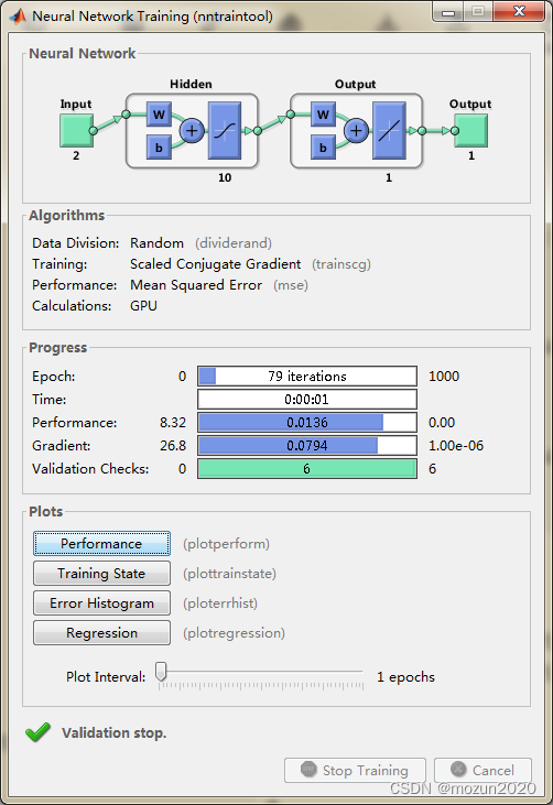
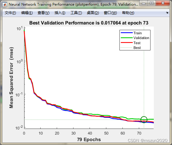
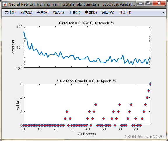
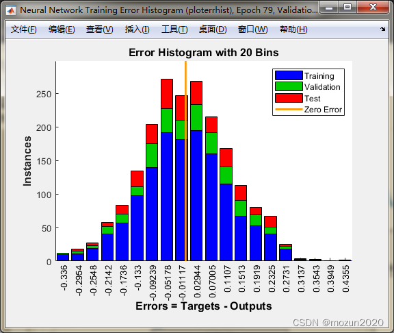
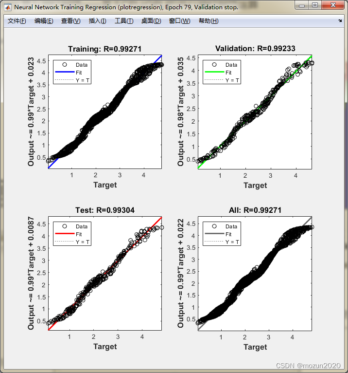
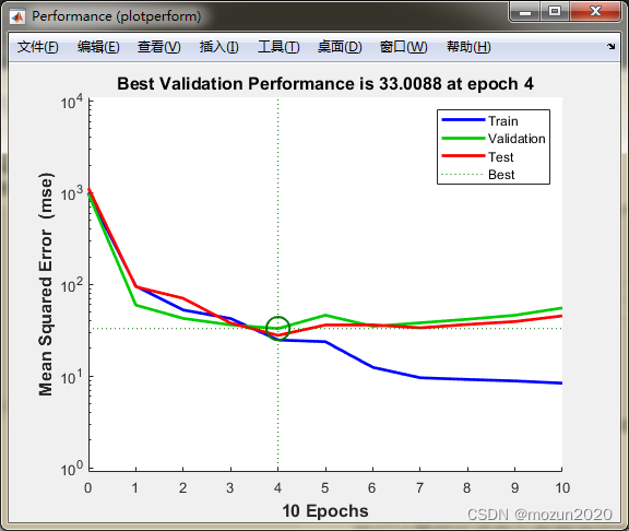
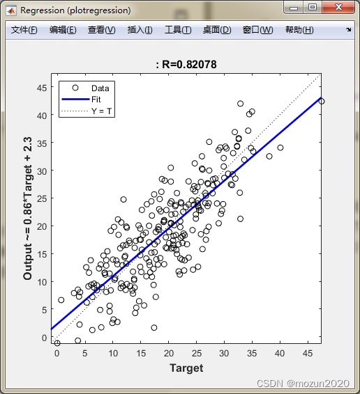
依次点击Plots中的Performance，Training State，Error Histogram，Regression可得到如下图示：

3. MATLAB 仿真示例二

选中并打开MATLAB当前文件夹视图中chapter42_2.m,

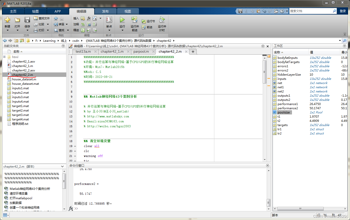
chapter42_2.m源码如下：

%%%%%%%%%%%%%%%%%%%%%%%%%%%%%%%%%%%%%%%%%%%%%%%%%%%%
%功能：并行运算与神经网络-基于CPU/GPU的并行神经网络运算
%环境：Win7，Matlab2015b
%Modi: C.S
%时间：2022-06-21
%%%%%%%%%%%%%%%%%%%%%%%%%%%%%%%%%%%%%%%%%%%%%%%%%%%%


%% Matlab神经网络43个案例分析

% 并行运算与神经网络-基于CPU/GPU的并行神经网络运算
% by 王小川(@王小川_matlab)
% http://www.matlabsky.com
% Email:sina363@163.com
% http://weibo.com/hgsz2003
 

%% 清空环境变量
clear all
clc
warning off
tic
%% 打开matlabpool
% matlabpool open
delete(gcp('nocreate'))
poolsize=parpool(2)

%% 加载数据
load bodyfat_dataset
inputs = bodyfatInputs;
targets = bodyfatTargets;

%% 创建一个拟合神经网络
hiddenLayerSize = 10;   % 隐藏层神经元个数为10
net = fitnet(hiddenLayerSize);  % 创建网络

%% 指定输入与输出处理函数(本操作并非必须)
net.inputs{
    
    1}.processFcns = {
    
    'removeconstantrows','mapminmax'};
net.outputs{
    
    2}.processFcns = {
    
    'removeconstantrows','mapminmax'};

%% 设置神经网络的训练、验证、测试数据集划分
net.divideFcn = 'dividerand';  % 随机划分数据集
net.divideMode = 'sample';  %  划分单位为每一个数据
net.divideParam.trainRatio = 70/100; %训练集比例
net.divideParam.valRatio = 15/100; %验证集比例
net.divideParam.testRatio = 15/100; %测试集比例

%% 设置网络的训练函数
net.trainFcn = 'trainlm';  % Levenberg-Marquardt

%% 设置网络的误差函数
net.performFcn = 'mse';  % Mean squared error

%% 设置网络可视化函数
net.plotFcns = {
    
    'plotperform','plottrainstate','ploterrhist', ...
  'plotregression', 'plotfit'};

%% 单线程网络训练
tic
[net1,tr1] = train(net,inputs,targets);
t1=toc;
disp(['单线程神经网络的训练时间为',num2str(t1),'秒']);

%% 并行网络训练
tic
[net2,tr2] = train(net,inputs,targets,'useParallel','yes','showResources','yes');
t2=toc;
disp(['并行神经网络的训练时间为',num2str(t2),'秒']);

%% 网络效果验证
outputs1 = sim(net1,inputs);
outputs2 = sim(net2,inputs);
errors1 = gsubtract(targets,outputs1);
errors2 = gsubtract(targets,outputs2);
performance1 = perform(net1,targets,outputs1);
performance2 = perform(net2,targets,outputs2);

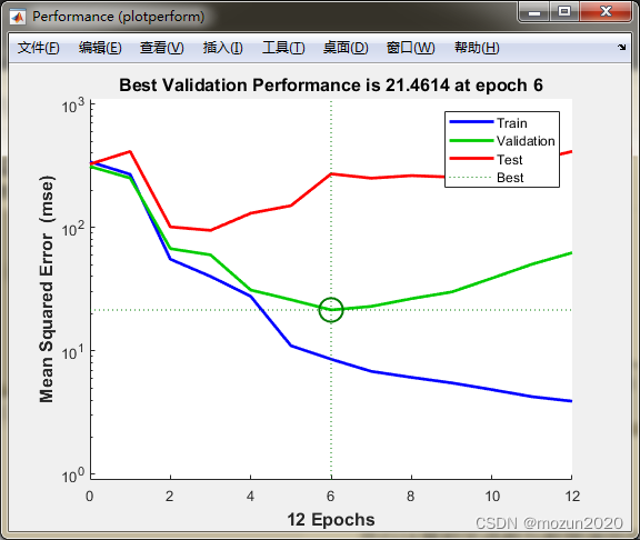
%% 神经网络可视化
figure, plotperform(tr1);
figure, plotperform(tr2);
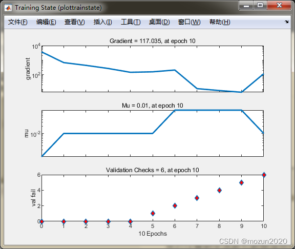
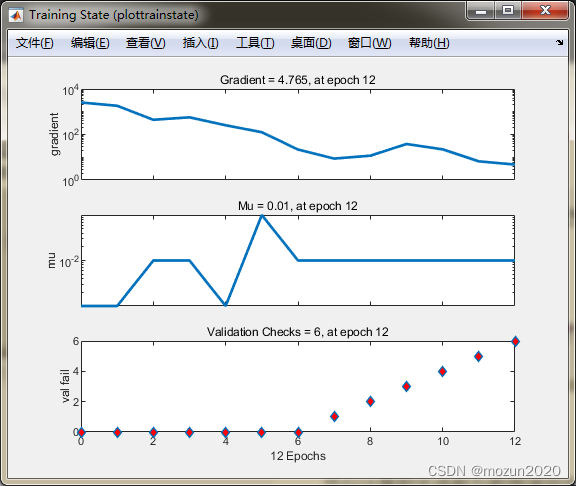
figure, plottrainstate(tr1);
figure, plottrainstate(tr2);
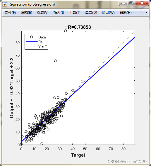
figure,plotregression(targets,outputs1);
figure,plotregression(targets,outputs2);
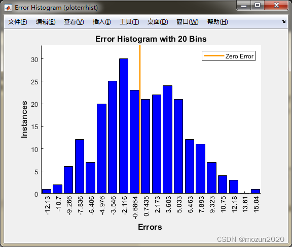
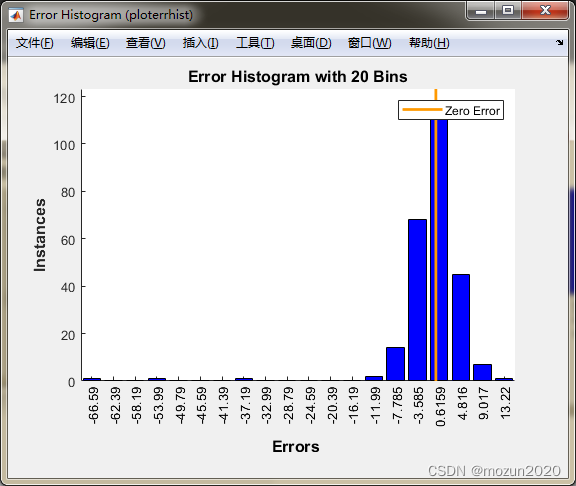
figure,ploterrhist(errors1);
figure,ploterrhist(errors2);
toc
% matlabpool close

点击“运行”，开始仿真，输出仿真结果如下：

Parallel pool using the 'local' profile is shutting down.
Starting parallel pool (parpool) using the 'local' profile ...
connected to 2 workers.

poolsize = 

 Pool - 属性: 

            Connected: true
           NumWorkers: 2
              Cluster: local
        AttachedFiles: {
    
    }
    AutoAddClientPath: true
          IdleTimeout: 30 minutes (30 minutes remaining)
          SpmdEnabled: true

单线程神经网络的训练时间为1.9707秒
 
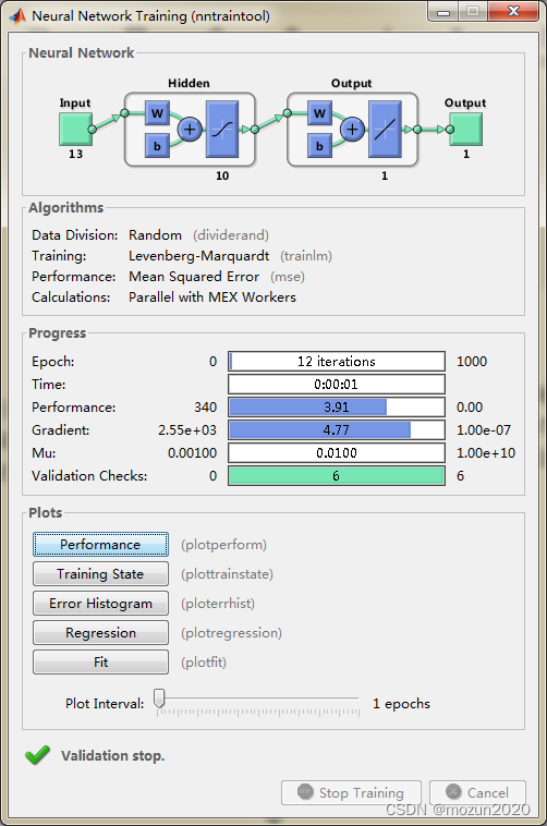
Computing Resources:
Parallel Workers:
  Worker 1 on 123-PC, MEX on PCWIN64
  Worker 2 on 123-PC, MEX on PCWIN64
 
并行神经网络的训练时间为4.4909秒

performance1 =

   26.4750


performance2 =

   50.1747

时间已过 12.766995 秒。

4. 小结

并行计算相关函数与数据调用在MATLAB2015版本之后都有升级，所以需要对源码进行调整再进行仿真，本文示例均根据机器情况与MATLAB版本进行适配。对本章内容感兴趣或者想充分学习了解的，建议去研习书中第四十二章节的内容。后期会对其中一些知识点在自己理解的基础上进行补充，欢迎大家一起学习交流。