【论文阅读】Learning Traffic as Images: A Deep Convolutional ... [将交通作为图像学习: 用于大规模交通网络速度预测的深度卷积神经网络]（3）

注: 阅读原文请转至link.

3. Empirical study（实验研究）

3.1. Data Description（数据描述）

 Beijing is the capital of China and one of the largest cities in the world. At present, Beijing is encircled by four two-way ring roads, that is, the second to fifth ring roads, and has about 10,000 taxis to serve its population of more than 21 million. These taxis are equipped with GPS devices that upload data approximately every minute. The uploaded data contain information, including car positions, recording time, moving directions, vehicle travel speeds, etc. The data were collected from 1 May 2015 to 6 June 2015 (37 days). These data are well-qualified probe data because the missing data accounts for less than 2.9%, and are properly remedied using spatiotemporal adjacent records. In this paper, data are aggregated into two-min intervals because data usually fluctuated over shorter time intervals, and the aggregation will cause data to be more stable and representative.
 北京是中国的首都，也是世界上最大的城市之一。目前，北京被四条双向环路环绕，即二环到五环，拥有约1万辆出租车，为2100多万人口服务。这些出租车配备了GPS设备，大约每分钟上传一次数据。上传的数据包含车辆位置、记录时间、移动方向、车辆行驶速度等信息。数据采集时间为2015年5月1日至6月6日(37天)。这些数据是非常合格的测试数据，因为缺失的数据占比小于2.9%，并且可以使用时空相邻记录进行适当的补救。在本文中，由于数据通常在较短的时间间隔内波动，所以将数据聚合为两分钟的间隔，这样会使数据更加稳定和具有代表性。

 In this paper, two sub-transportation networks, i.e., the second ring (labeled as Network 1) and north-east transportation network (labeled as Network 2) of Beijing, are selected to demonstrate the proposed method. The two networks differ in network size and topology complexity, as shown in Figure 3. Network 1 consists of 236 road sections for aggregating GPS data, all of which are one-way roads. Network 2 consists of 352 road sections, including two-way and crossroads. The selected networks represent different road topologies and structures and, thus, can be used to better evaluate the effectiveness of the proposed CNN traffic prediction algorithm.
 本文以北京市二环(标记为网络1)和东北交通网络(标记为网络2)两个子交通网络为例，对该方法进行了验证。这两个网络在网络大小和拓扑复杂度方面存在差异，如图3所示。网络1由236个路段组成，用于聚合GPS数据，均为单行道。网络2由352个路段组成，包括双向路段和十字路口路段。所选择的网络代表了不同的道路拓扑和结构，因此，可以用来更好地评估所提出的CNN交通预测算法的有效性。

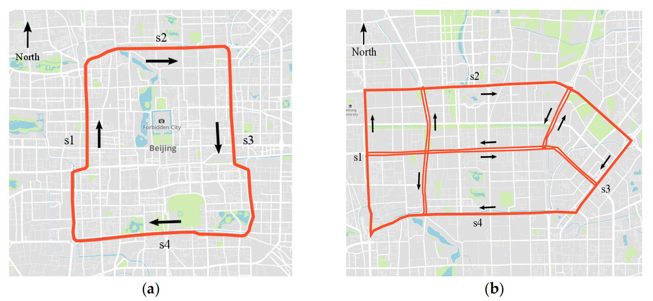
Figure 3. Two sub-transportation networks for testing: (a) Network 1, the second ring of Beijing; and (b) Network 2, a network in Northeast Beijing
图3. 2个待测试的子交通网络: (a) 网络1，北京二环; (b) 网络2，北京东北地区的网络

 Four prediction tasks are performed to test the CNN algorithm in predicting network-wide traffic speeds. These tasks differ in prediction time spans, i.e., short-term and long-term predictions, and in input information, i.e., prediction using abundant information and prediction using limited information. The four tasks are listed as follows:
 Task 1: 10-min traffic prediction using last 30-min traffic speeds;
 Task 2: 10-min traffic prediction using last 40-min traffic speeds;
 Task 3: 20-min traffic prediction using last 30-min traffic speeds; and
 Task 4: 20-min traffic prediction using last 40-min traffic speeds.
 通过四个预测任务来测试CNN算法在预测网络范围内的流量速度。这些任务的不同之处在于预测时间跨度，即短期预测和长期预测; 输入信息，即利用丰富信息的预测和利用有限信息的预测。四项任务如下:
 任务1:利用过去30分钟的交通速度预测接下来10分钟的交通;
 任务2:利用过去40分钟的交通速度预测接下来10分钟的交通;
 任务3:利用过去30分钟的交通速度预测接下来20分钟的交通;
 任务4:使用过去40分钟的交通速度预测接下来20分钟的交通。

 In the four tasks, the capabilities and effectiveness of CNN in predicting large-scale transportation network speed can be validated by calculating and comparing the MSEs of CNN.
 在这四个任务中，可以通过计算和比较CNN的MSEs来验证CNN预测大规模交通网络速度的能力和有效性。

3.2 Time-Space Image Generation（时空图像生成）

 In terms of time-space matrix representation, the goal is to transform spatial relations of the traffic in a transportation network into linear representations. The matrix is straightforward in Network 1 because connected road sections in the ring road can be easily straightened. For Network 2, straightening the road sections into a straight line while maintaining the complete spatial relations of these sections is impossible. A compromise is to segment the network into straight lines and lay road sections in order on these lines. Consequently, in Network 2, only a linear spatial relation on straight lines can be captured. However, complex and network-wide relations of traffic speeds in Network 2 can still be learned because the CNN can learn features from local connections and compose these features into high-level representations [32] , [36] . Regarding Network 2, the CNN learns the relations of traffic roads from segmented road sections and composes these relations into network-wide relations.
 在时空矩阵表示方面，目标是将交通网络中交通的空间关系转换为线性表示。网络1中的矩阵是直接的，因为环路中连接的路段可以很容易地拉直。对于网络2，不可能在保持路段完整空间关系的情况下，将路段矫直成一条直线。一种折衷办法是将网络分割成直线，并在这些直线上按顺序铺设路段。因此，在网络2中，只能捕捉直线上的线性空间关系。然而，由于CNN可以从局部连接中学习特征，并将这些特征合成为高级表示形式，因此网络2中复杂的、全网络范围的流量速度关系仍然可以学习 [32]，[36] 。在网络2中，CNN从分割的路段中学习交通道路的关系，并将这些关系组合成全网络关系。

 After using a time-space matrix as the channel of an image and representing everyday traffic speeds of the network in an image, 37 images, each corresponding to a day, can be generated for Networks 1 and 2, respectively. Sample images of Networks 1 and 2 on 26 May 2015 are shown in Figure 4. The y-labels of Figure 4, i.e., s1, s2, s3, s4, and other, are road sections shown in Figure 3. The images show rich traffic information, such as the most congested traffic areas, in red regions, and typical congestion propagation patterns, i.e., oscillating congested traffic (OCT) and pinned localized clusters (PLC). A more specific explanation on these traffic patterns can be found in the study by Schönhof and Helbing [37] . Such rich information cannot be well learned by a simple ANN. Thus, a more effective algorithm is necessary.
 用一个时空矩阵作为图像的通道，用一幅图像表示网络每天的流量速度，可以分别为网络1和网络2生成37幅图像，每幅图像对应一天。网络1和网络2在2015年5月26日的样图如图4所示。图4的y标签为s1、s2、s3、s4、other，为图3所示路段。图中显示了丰富的交通信息，如红色区域为最拥挤的交通区域，以及典型的交通拥堵传播模式，即oscillating congested traffic (OCT) 和 pinned localized clusters (PLC)。关于这些交通模式的更具体的解释可以在Schönhof和Helbing [37] 的研究中找到。这样丰富的信息不能通过一个简单的人工神经网络很好地学习。因此，需要一种更有效的算法。

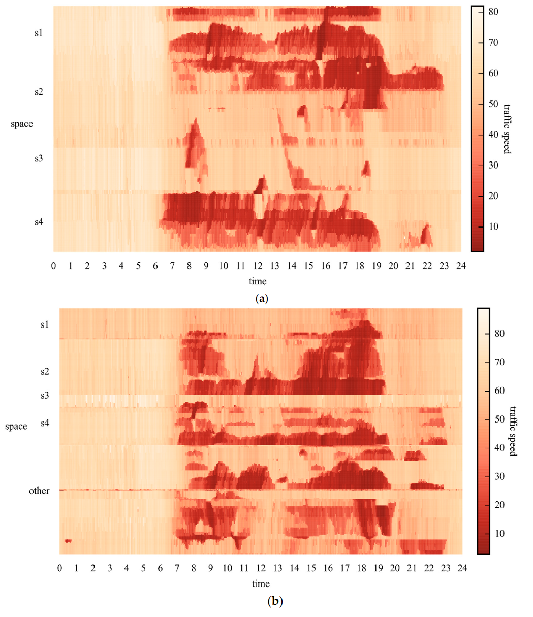
Figure 4. Sample images with spatiotemporal traffic speeds for (a) Network 1; and (b) Network 2.
图4. (a) 网络1的时空交通速度样本图像; (b) 网络2的时空交通速度样本图像

扫描二维码关注公众号，回复： 14228709 查看本文章

3.3. Turning Up CNN Parameters（CNN参数更新）

 Two critical factors should be considered when implementing the structure of a CNN: (a) hyperparameters concerned with convolutional and pooling layers, such as convolutional filter size, polling size, and polling method; and (b) depth of the CNN.
 在实现CNN的结构时，需要考虑两个关键因素:(a)与卷积和池化层有关的超参数，如卷积滤波器大小、轮询大小和轮询方法; (b) CNN的深度。

 First, the selection of hyperparameters relies on experts’ experience. No general rules can be applied directly. Two well-known examples can be referred. One is LeNet, which marked the beginning of the development of CNN [38] , and the other is AlexNet, which won the image classification competition ImageNet in 2010 [31] . Based on the parameter settings of LeNet and AlexNet, we select convolutional filters of size $(3,3)$ and max poolings of size $(2,2)$ for the example networks.
 首先，超参数的选择依赖于研究人员的经验。没有任何一般规则可以直接适用。可以参考两个著名的例子。一个是LeNet，它标志着CNN [38] 发展的开始，另一个是AlexNet，它赢得了2010年ImageNet的图像分类比赛 [31] 。根据LeNet和AlexNet的参数设置，我们为示例网络选择大小为$(3,3)$的卷积滤波器和大小为$(2,2)$的最大poolings。

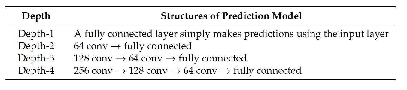
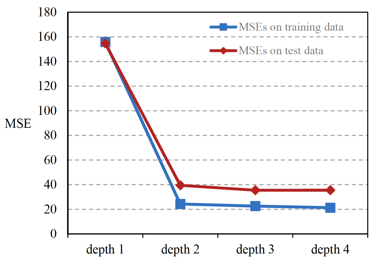
 Second, the depth of CNN should be neither too large nor too small [39] and, thus, CNN is capable of learning much more complex relations while maintaining the convergence of the model. Different values, from small to large, are assigned to test the CNN model until the incremental benefits are diminished and the convergence becomes difficult in determining a proper value for the depth of the model. The structures of the CNN in different depths are listed in Table 1, where each convolutional layer is followed by a pooling layer, and the numbers represent quantities of convolutional filters in the layer. Obviously, the depth-1 network is a fully connected layer that transforms inputs into predictions, whereas the three other networks first extract spatiotemporal traffic features from the input image using convolutional and pooling layers, and then make predictions based on them. In the experiments, the 40 min historical traffic speeds are used to predict the following 10 min traffic speeds. In model training, 21,600 samples on the first 30 days are used, and in model validation, 5040 samples in the following seven days are used. The results are shown as Figure 5, which shows that adding depth to the CNN model significantly reduces MSEs on the testing data. As a result, a depth-4 CNN model achieves the lowest MSEs on the training and testing data, which are 21.3 and 35.5, respectively. Therefore, the depth-4 model is adopted for experiments in this paper.
 其次，CNN的深度不应该太大也不应该太小[39]，这样，CNN在保持模型收敛的同时，可以学习更加复杂的关系。不同的值按照从小到大被分配来测试CNN模型，直到参数更新效益减小并且模型难以收敛，以此方法来确定出一个合适的值作为模型的深度。不同深度CNN的结构如表1所示，其中每个卷积层后面都有一个池化层，数字表示该层中卷积滤波器的数量。显然，depth-1网络是一个将输入转换为预测的全连接层，而其他三个网络首先使用卷积层和池化层从输入图像中提取时空流量特征，然后基于这些特征进行预测。在实验中，利用40分钟的历史交通速度来预测接下来10分钟的交通速度。在模型训练中，使用了前30天的21600个样本，在模型验证中，使用了后7天的5040个样本。结果如图5所示，从图中可以看出，在CNN模型中加入深度显著降低了对测试数据的MSEs。因此，depth-4 CNN模型在训练数据和测试数据上获得的MSEs最低，分别为21.3和35.5。因此，本文采用depth-4模型进行实验。

Table 1. Different depths for CNN. 表1. 不同深度的CNN模型

Figure 5. Results of CNN in different depths. 图5. 不同深度CNN的测试结果

• 注：关于均方误差MSE的讲解请看通俗易懂讲解均方误差MSE。

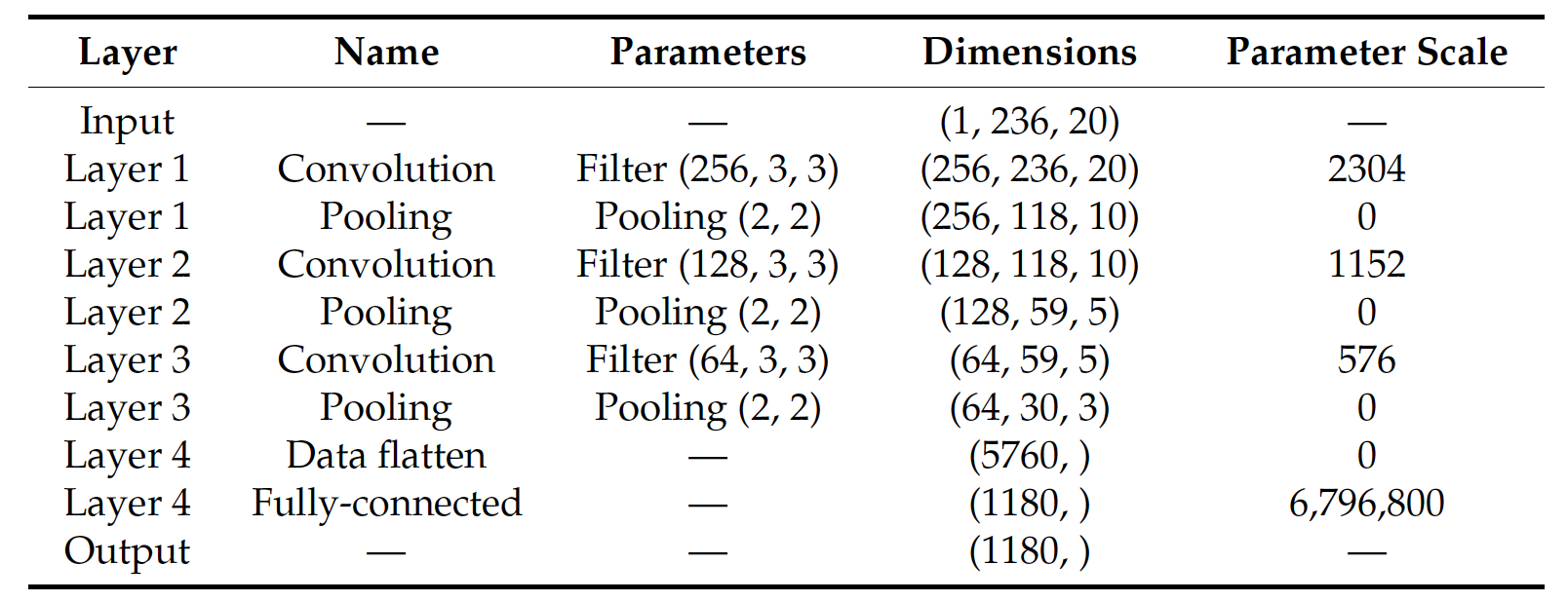
 The details of the depth-4 CNN are listed in Table 2. The model input has three dimensions $(1,236,20)$, where the first number indicates that the input image has one channel, the second number represents the total number of road sections in Network 1, and the third number refers to the input time span, which is 20 time units. Convolutional layers consecutively transform the number of channels into 256, 128, and 64 with the corresponding quantity of convolutional filters, respectively. At the same time, pooling layers consecutively downsample the input window to $(118,10)$, $(59,5)$, and $(30,3)$. The output dimensions in layer 6 are $(64,30,3)$, which are then flattened into a vector with a dimension of 5760. The vector is finally transformed into the model output with a dimension of 1180 through a fully-connected layer.
 depth-4 CNN的详细信息如表2所示。模型输入有三个维度$(1,236,20)$，其中第一个数字表示输入图像有一个通道，第二个数字表示网络1的总路段数，第三个数字表示输入的时间跨度，为20个时间单位。卷积层依次将信道数转换为256、128、64，并分别对应卷积滤波器的数量。同时，池化层连续向下采样输入窗口到$(118,10)$，$(59,5)$和$(30,3)$。第6层的输出维度为$(64,30,3)$，然后将其扁平化为一个维度为5760的向量。最后通过全连通层将向量转换为1180维的模型输出。

Table 2. Hyperparameters of the CNN. 表2. CNN的超参数

 Early stopping criterion is applied to prevent the model from overfitting. Model overfitting is a situation where model training does not improve prediction accuracy of the CNN on validation data, although it improves the prediction accuracy of the CNN on testing data. The model should stop training when it begins to overfit. Early stopping is the most common and effective procedure to avoid overfitting issues [40] . This method works in the phase of model training, and early stopping occurrence records losses of the model on the validation dataset. After model training in each epoch, it checks if the losses increase or remain unchanged. Finally, if true and no sign of improvements are observed within a specific number of epochs, model training will be terminated.
 采用早停法防止模型过拟合。模型过拟合是指模型训练虽然提高了CNN对测试数据的预测精度，但并没有提高CNN对验证数据的预测精度。当模型开始过度拟合时，应该停止训练。早期停止是避免过度拟合问题最常见和有效的方法 [40] 。该方法工作在模型训练阶段，早期停止发生记录模型在验证数据集上的丢失。在每个epoch进行模型训练后，检查损失是否增加或保持不变。最后，如果是真的，并且在特定的时间段内没有观察到任何改善的迹象，则将终止模型训练。

3.4 Results and Comparison（结果和比较）

 In order to test the performance of the proposed algorithm, four prevailing statistical algorithms and three deep learning based algorithms are chosen for comparison. OLS is the basic regression algorithm and taken as the benchmark. KNN performs regression using the nearest points. Random forest (RF) makes predictions based on branches of decision trees. ANN represents the traditional neural network and attempts to learn features through hidden layers. SAE is a neural network consisting of multiple layers of autoencoders, where model inputs are encoded into dense or sparse representations before being fed into the next layer [28] . RNN can learn the features by unfolding the time series and capturing the pattern through its shared parameters and hidden states at each time step [27] . LSTM NN is an extension of RNN and becomes popular since the architecture can deal with long-term memories and avoid vanishing gradient issues that traditional RNNs suffer from [30] . These algorithms differ in their ability to predict traffic speeds for multiple road sections in a network. OLS, KNN, and RF can only output the traffic prediction on each link at a time. Hence, to predict network-wide traffic speeds, a large number of models have to be developed. In contrast, ANN, SAE, RNN and LSTM NN can yield network-wide traffic speeds in one model with multi-step outputs. As for the ability to take spatial relations into account, all algorithms treat traffic speeds in different sections as independent sequences and cannot learn spatial relations among sections. Moreover, KNN is configured to use the 10 nearest points. RF is set up to generate 10 decision trees. ANN, RNN, and LSTM NN are optimized to contain three hidden layers with 1000 hidden units in each layer. SAE is tuned up to form up three autoencoder layers with 3000, 2500, and 2000 hidden units in the three layers, respectively.
 为了测试所提算法的性能，本文选取了四种流行的统计算法和三种基于深度学习的算法进行比较。OLS是最基本的回归算法，以OLS为基准。KNN使用最近的点执行回归。随机森林(Random forest, RF)基于决策树的分支进行预测。ANN代表传统的神经网络，试图通过隐藏层来学习特征。SAE是一个由多层自动编码器组成的神经网络，其中模型输入被编码成密集或稀疏表示，然后被送入下一层 [28] 。RNN可以通过对时间序列展开来学习特征，并通过每个时间步长 [27] 的共享参数和隐藏状态来捕获模式。LSTM神经网络是RNN的一种扩展，由于其结构能够处理长期记忆，并且避免了传统RNN在 [30] 中存在的梯度消失问题，因此得到了广泛的应用。这些算法在预测网络中多个路段的交通速度的能力上有所不同。OLS、KNN和RF在同一时间只能输出每条链路上的流量预测。因此，要预测网络范围内的交通速度，需要开发大量的模型。相比之下，人工神经网络、SAE、RNN和LSTM神经网络可以在一个多步输出的模型中给出全网络的交通速度。在考虑空间关系的能力方面，所有算法都将不同路段的交通速度视为独立序列，无法学习路段之间的空间关系。此外，KNN被配置为使用最近的10个点。建立RF生成10棵决策树。将ANN、RNN和LSTM三种神经网络进行优化，使其包含三个隐含层，每层隐含单元1000个。SAE将自动编码器分为3层，分别包含3000、2500和2000个隐藏单元。

 Table 3 and Figure 6 show the results of different algorithms and CNN when applied to Networks 1 and 2 in four different prediction tasks. The results show that, in all circumstances, the CNN algorithm outperforms other algorithms on testing data, implying that CNN can be better generalized to new data samples. One possible reason is that OLS, KNN, RF, and ANN treat traffic speeds in each section as independent sequences and assumes that traffic speeds in each section are self-affected. This assumption ignores spatial relations among road sections in the network and neglects the important mutual effect of adjacent sections or deeper traffic features. The existing deep learning architectures, i.e., SAE, RNN, and LSTM NN, are also inferior to CNN. This is probably because the majority of existing deep learning-based traffic prediction algorithms cannot incorporate spatial information from the perspective of a network, whereas there exists a strong correlation between multiple congestion bottlenecks [41] .
 表3和图6显示了不同算法和CNN在四种不同预测任务下应用于network1和network2的结果。结果表明，在所有情况下，CNN算法在测试数据上的表现都优于其他算法，这意味着CNN可以更好地推广到新的数据样本。一个可能的原因是OLS、KNN、RF和ANN将每个路段的交通速度视为独立序列，并假设每个路段的交通速度是自影响的。这种假设忽略了路网中各路段之间的空间关系，忽略了相邻路段或更深层次交通特征之间的重要相互影响。现有的深度学习体系结构SAE、RNN、LSTM神经网络也不如CNN。这可能是因为现有的基于深度学习的流量预测算法大多不能从网络的角度整合空间信息，而多个拥塞瓶颈 [41] 之间存在很强的相关性。

 Long-term predictions using CNN can also be validated by comparing the results of tasks 1–4. Usually, when the input time-span is fixed, long-term predictions achieve higher MSEs than short-term predictions, which implies that making long-term predictions is more difficult than making short-term predictions.
 使用CNN的长期预测也可以通过比较任务1-4的结果来验证。通常，当输入的时间跨度是固定的，长期预测比短期预测获得更高的MSEs，这意味着进行长期预测比进行短期预测更困难。

Table 3. Prediction performance (MSE) of the CNN and other algorithms. 表3. CNN与其它算法算法的预测性能(MSE)
Figure 6. Results of different algorithms: (a) MSEs on Network 1; and (b) MSEs on Network 2. 图6. 不同算法的结果: (a) 网络1上的MSEs; (b) 网络2上的MSEs

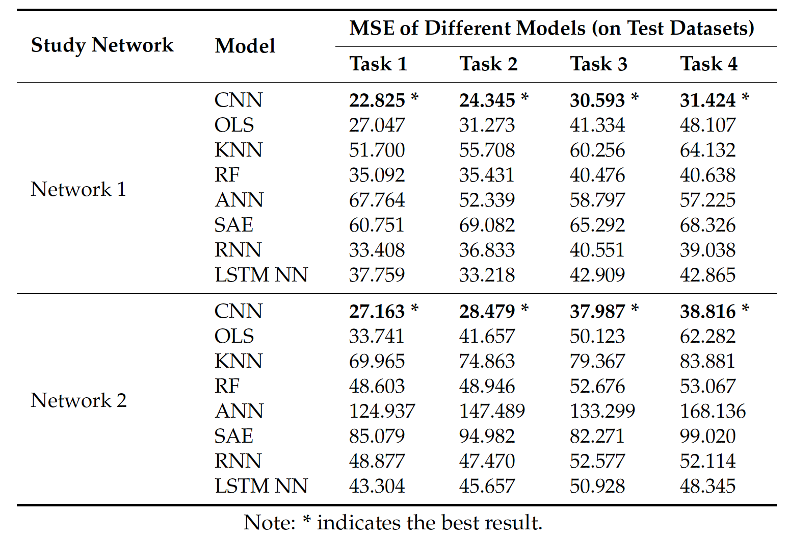
 We further converted the predicted traffic speeds into three categories of traffic states: heavy traffic (0–20 km/h), moderate traffic (20–40 km/h), and free-flow traffic (>40 km/h). Such a presentation is preferable for travelers to plan their routes. The performance of different algorithms in terms of prediction accuracy is presented in Table 4. The results show that CNN achieves the highest prediction accuracies in all circumstances with an average prediction accuracy of 0.931, followed by OLS (0.917) and RF (0.904), which implies that it is necessary to incorporate spatiotemporal features from a network-wide perspective.
 我们进一步将预测的交通速度分为三类交通状态:繁忙交通状态(0-20 km/h)、中等交通状态(20-40 km/h)和自由交通状态(>40 km/h)。这样的展示对于旅行者计划他们的路线是更好的。不同算法在预测精度方面的性能如表4所示。结果表明，在所有情况下，CNN的预测精度最高，平均预测精度为0.931，其次是OLS(0.917)和RF(0.904)，这意味着有必要从网络的角度整合时空特征。

Table 4. Prediction performance (accuracy) of the CNN and other algorithms. 表4. CNN等算法的预测性能(准确率)。

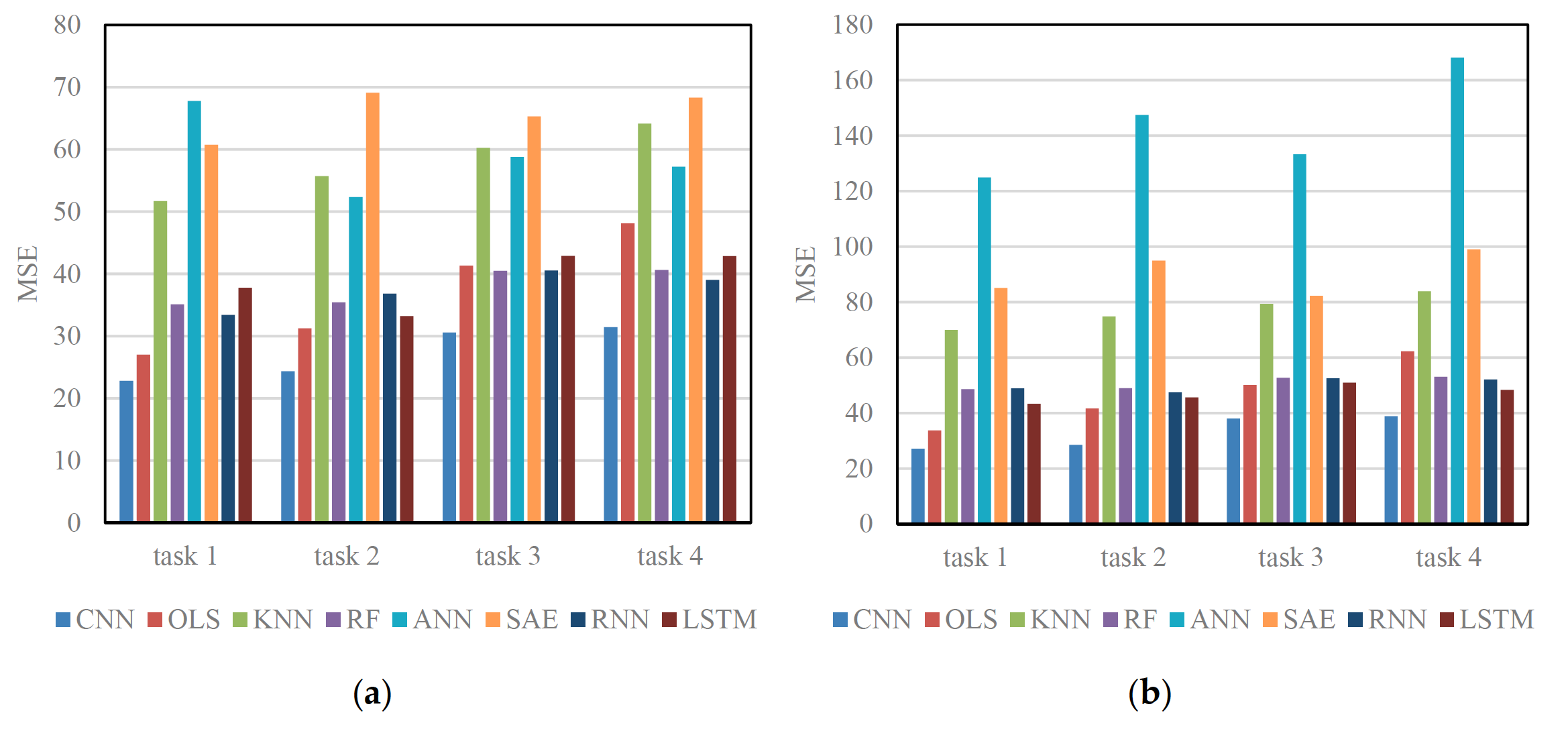
 Figure 7 shows training time of different algorithms on Networks 1 and 2. OLS, KNN, and ANN train the model more efficiently than the CNN because these algorithms have simple structures and are easy to train. However, these algorithms make significant trade-offs between their training efficiency and prediction accuracy. Other deep learning architectures, i.e., SAE, RNN and LSTM NN, require less training time than the CNN. This is primarily due to the fact that the CNN applies a large quantity of convolutional kernels to each image in order to extract extensive network-wide spatiotemporal traffic features. As for RF, it takes about nine hours to train and obtains much better results, but these results are still inferior to the CNN. RF may fail when applied to a larger-scale transportation network in real-time. Therefore, when both training efficiency and accuracy are considered, the proposed CNN outperforms the other algorithms.
 图7显示了不同算法在网络1和网络2上的训练时间。OLS、KNN和ANN对模型的训练比CNN更有效，因为这些算法结构简单，易于训练。然而，这些算法在训练效率和预测精度之间做了重大的权衡。其他的深度学习体系结构，如SAE、RNN和LSTM神经网络，比CNN需要更少的训练时间。这主要是由于CNN对每幅图像应用了大量的卷积核，以提取广泛的网络范围内的时空交通特征。对于RF，它需要大约9个小时的训练，并且得到了更好的结果，但是这些结果仍然不如CNN。在大规模的实时传输网络中，射频可能会出现故障。因此，在兼顾训练效率和准确性的情况下，本文提出的CNN算法优于其他算法。

Figure 7. Training time of different algorithms: (a) training time on Network 1; and (b) training time on Network 2.
图7. 不同算法的训练时间: (a) 网络1上的训练时间; (b) 网络2的培训时间。

 Based on the above discussion, useful conclusions can be yielded as follows:

• The CNN outperforms other algorithms on testing data with an average accuracy improvement of 42.91%, which implies that it is important to learn spatiotemporal features through the proposed scheme.
• The CNN trains the model within a reasonable time, but still achieves the most accurate predictions in all circumstances. As for RF, it consumes much more training time compared with CNN and receives lower accurate predictions. The OLS, KNN, and ANN train the model much faster but only yield unusable prediction results. Compared with other deep learning architectures employed, i.e., SAE, RNN and LSTM NN, the CNN trains the model much slower, but it achieves more accurate prediction results through extensive spatiotemporal features.
• The CNN performs best in long-term predictions compared with other algorithms, although making long-term traffic predictions is usually more difficult than making short-term predictions.
   综上所述，可以得出以下有用的结论:
• CNN在测试数据上的性能优于其他算法，平均准确率提高了42.91%，这意味着通过本文提出的方案学习时空特征是重要的。
• CNN在合理的时间内训练模型，但仍然在所有情况下实现最准确的预测。对于RF来说，与CNN相比，它消耗了更多的训练时间，并且预测的准确率较低。OLS、KNN和ANN训练模型的速度快得多，但只产生不可用的预测结果。与采用的其他深度学习架构，如SAE、RNN和LSTM神经网络相比，CNN训练模型的速度要慢得多，但通过广泛的时空特征获得了更准确的预测结果。
• 与其他算法相比，CNN在长期预测方面表现最好，尽管进行长期流量预测通常比进行短期预测更难。

4. Conclusions（结论）

 Deep learning methods are widely used in the domain of image processing with satisfactory results, since deep learning architectures usually have deeper construction and depict more complex nonlinear functions than other neural networks [25,27,30,39] . However, limited studies have addressed spatiotemporal relations among road sections in transportation networks. Spatiotemporal relations are important traffic characteristics. A better understanding of these relations will improve the accuracy of traffic prediction.
 深度学习方法在图像处理领域得到了广泛的应用，并取得了令人满意的结果，因为深度学习体系结构通常比其他神经网络具有更深入的构造和描述更复杂的非线性函数 [25,27,30,39] 。然而，关于交通网络中路段之间的时空关系的研究还很有限。时空关系是重要的交通特征。更好地理解这些关系将提高交通预测的准确性。

 This paper proposes an image-based traffic speed prediction method that can extract abstract spatiotemporal traffic features in an automatic manner to learn spatiotemporal relations. The method contains two main procedures. The first procedure involves converting network traffic to images that represent time and space dimensions of a transportation network as two dimensions of an image. Spatiotemporal information can be preserved because surrounding road sections are adjacent in the image. The second procedure is to employ the deep learning architecture of a CNN to the image for traffic prediction. CNN has attained significant success in computer vision and performs well in image-learning tasks [31] . In this transportation prediction problem, the CNN shares the following important properties: (a) spatiotemporal features of the transportation network can be extracted automatically because of the implementation of convolutional and pooling layers of CNN; thus, the need for manual feature selection can be avoided; (b) the CNN represents network-wide traffic information of high-level features that are then used to create network-wide traffic speed predictions; and (c ) the CNN can be generalized to large transportation networks because it shares weights in convolutional layers and employs the pooling mechanism. Two empirical transportation networks and four prediction tasks are considered to test the applicability of the proposed method. The results show that the proposed method outperforms OLS, KNN, ANN, RF, SAE, RNN, and LSTM NNs with an average accuracy promotion of 42.91%. The training time of the proposed method is acceptable because the proposed method achieves the best MSEs on testing data in seven (out of eight) tasks and takes much less training time than RF, which achieves the best MSEs on training data and achieves the second-best prediction accuracy on testing data.
 本文提出了一种基于图像的交通速度预测方法，该方法能够自动提取抽象的时空交通特征，学习时空关系。该方法包含两个主要的过程。第一个过程涉及到将网络流量转换为图像，将交通网络的时间和空间维度表示为图像的两个维度。由于在图像中周围的路段是相邻的，因此可以保存时空信息。第二步是将CNN的深度学习架构应用到图像中进行交通预测。CNN在计算机视觉方面取得了巨大的成功，在图像学习任务 [31] 中表现良好。在这个交通预测问题中，CNN具有以下重要的特性: (a) 由于CNN实现了卷积层和池化层，可以自动提取交通网络的时空特征;因此，可以避免手动选择特征; (b) CNN代表高级别特征的全网交通信息，然后用于创建全网交通速度预测; © 由于CNN在卷积层中共享权值，并采用池化机制，因此可以推广到大型运输网络。考虑两个经验交通网络和四个预测任务来测试所提方法的适用性。结果表明，该方法优于OLS、KNN、神经网络、RF、SAE、RNN和LSTM神经网络，平均准确率提高了42.91%。该方法的训练时间是可以接受的,因为该方法在七（八）个任务上测试数据的MSE分数达到了最好，并且比在测试数据中达到最好的MSE分数和第二好的预测精度的RF模型用了更少的训练时间。

 The proposed method has some possible interesting extensions. For example, in the second procedure, other models, such as the combination of CNN and LSTM NN, would be an interesting attempt. Specifically, CNN can first extract abstract traffic features from a transportation network. The feature vectors can be fed into the LSTM NN model for prediction accuracy enhancement.
 所提出的方法有一些可能的有趣的扩展。例如，在第二个过程中，其他的模型，如CNN和LSTM 神经网络的结合，将是一个有趣的尝试。具体来说，CNN可以首先从交通网络中提取出抽象的交通特征。将特征向量输入LSTM神经网络模型，提高预测精度。

参考文献

25. Huang, W.; Song, G.; Hong, H.; Xie, K. Deep Architecture for Traffic Flow Prediction: Deep Belief Networks With Multitask Learning. IEEE Trans. Intell. Transp. Syst. 2014, 15, 2191–2201.

27. Ma, X.; Yu, H.; Wang, Y.; Wang, Y. Large-scale transportation network congestion evolution prediction using deep learning theory. PLoS ONE 2015, 10, e0119044.

28. Lv, Y.; Duan, Y.; Kang, W.; Li, Z.; Wang, F.Y. Traffic Flow Prediction With Big Data: A Deep Learning Approach. IEEE Trans. Intell. Transp. Syst. 2014, 16, 1–9.

30. Ma, X.; Tao, Z.; Wang, Y.; Yu, H.; Wang, Y. Long short-term memory neural network for traffic speed prediction using remote microwave sensor data. Transp. Res. Part C Emerg. Technol. 2015, 54, 187–197.

31. Krizhevsky, A.; Sutskever, I.; Hinton, G.E. ImageNet Classification with Deep Convolutional Neural Networks. In Proceedings of the 25th International Conference on Neural Information Processing Systems, Lake Tahoe, NV, USA, 3–6 December 2012.

32. Oquab, M.; Bottou, L.; Laptev, I.; Sivic, J. Learning and Transferring Mid-level Image Representations Using Convolutional Neural Networks. In Processedings of the 2014 IEEE Conference on Computer Vision and Pattern Recognition, Columbus, OH, USA, 23–28 June 2014; pp. 1717–1724.

36. LeCun, Y.; Bengio, Y. Convolutional networks for images, speech, and time series. In The Handbook of Brain Theory and Neural Networks; MIT Press: Cambridge, MA, USA, 1998; Volume 3361, pp. 255–258.

37. Schönhof, M.; Helbing, D. Empirical Features of Congested Traffic States and Their Implications for Traffic Modeling. Transp. Sci. 2007, 41, 135–166.

38. Lecun, Y.; Boser, B.; Denker, J.S.; Henderson, D.; Howard, R.E.; Hubbard, W.; Jackel, L.D. Backpropagation applied to handwritten zip code recognition. Neural Comput. 1869, 1, 541–551.

39. Lv, Y.; Duan, Y.; Kang, W.; Li, Z.; Wang, F.-Y. Traffic flow prediction with big data: A deep learning approach. IEEE Trans. Intell. Transp. Syst. 2015, 16, 865–873.

40. Sarle, W.S. Stopped Training and Other Remedies for Overfitting. In Proceedings of the 27th Symposium on the Interface of Computing Science and Statistics, Fairfax, VA, USA, 21–24 June 1995; pp. 352–360.

41. Kerner, B.S.; Rehborn, H.; Aleksic, M.; Haug, A. Recognition and tracking of spatial-temporal congested traffic patterns on freeways. Transp. Res. Part C Emerg. Technol. 2004, 12, 369–400.