【论文阅读】Spatio-Temporal Graph Convolutional Networks:...Traffic Forecasting[时空图卷积网络:用于交通预测的深度学习框架]（3）

原文地址：https://transport.ckcest.cn/Search/get/298151?db=cats_huiyi_jtxs

3. Proposed Model（模型）

3.1 Network Architecture（网络结构）

In this section, we elaborate on the proposed architecture of spatio-temporal graph convolutional networks (STGCN). As shown in Figure 2, STGCN is composed of several spatio- temporal convolutional blocks, each of which is formed as a “sandwich” structure with two gated sequential convolution layers and one spatial graph convolution layer in between. The details of each module are described as follows.
在本节中，我们详细阐述了提出的时空图卷积网络(STGCN)架构。如图2所示，STGCN由多个时空卷积块组成，每个卷积块形成一个“三明治”结构，中间有两个门控顺序卷积层和一个空间图卷积层。各模块的详细信息如下所示。

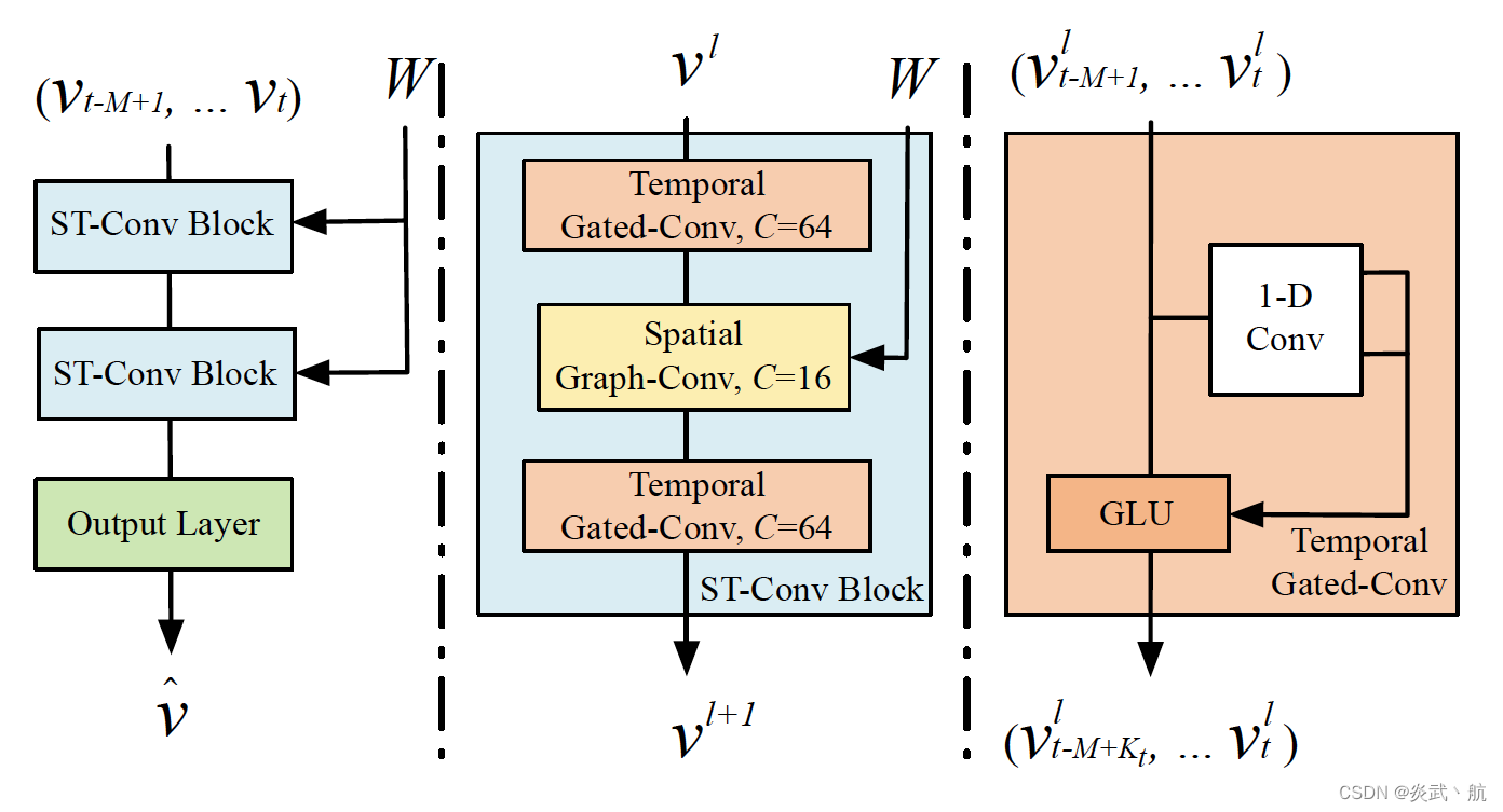
Figure 2: Architecture of spatio-temporal graph convolutional net- works. The framework STGCN consists of two spatio-temporal convolutional blocks (ST-Conv blocks) and a fully-connected output layer in the end. Each ST-Conv block contains two temporal gated convolution layers and one spatial graph convolution layer in the middle. The residual connection and bottleneck strategy are applied inside each block. The input $v_{t-M+1},\dots ,v_t$ is uniformly processed by ST-Conv blocks to explore spatial and temporal dependencies coherently. Comprehensive features are integrated by an output layer to generate the final prediction $\hat{v}$.
图2: 时空图卷积网络架构。STGCN框架由两个时空卷积模块(ST-Conv模块)和一个全连接的输出层组成。每个ST-Conv模块包含两个时间门控卷积层和中间的一个空间图卷积层。在每个块内部应用剩余连接和瓶颈策略。ST-Conv块对输入 $v_{t-M+1},\dots ,v_t$ 进行统一处理，以一致性地探索空间和时间相关性。综合功能被输出层集成，以生成最终的预测 $\hat{v}$ 。

3.2 Graph CNNs for Extracting Spatial Features（用于提取空间特征的图CNN）

The traffic network generally organizes as a graph structure. It is natural and reasonable to formulate road networks as graphs mathematically. However, previous studies neglect spatial attributes of traffic networks: the connectivity and globality of the networks are overlooked, since they are split into multiple segments or grids. Even with $2$-D convolutions on grids, it can only capture the spatial locality roughly due to compromises of data modeling. Accordingly, in our model, the graph convolution is employed directly on graph-structured data to extract highly meaningful patterns and features in the space domain. Though the computation of kernel $\Theta$ in graph convolution by Eq. (2) can be expensive due to $O(n^2)$ multiplications with graph Fourier basis, two approximation strategies are applied to overcome this issue.
交通网络通常以图的形式呈现。用数学的方法来表示路网是自然而合理的。然而，以往的研究忽略了交通网络的空间属性: 由于将交通网络划分为多个区段或网格，忽视了交通网络的连通性和全局性。即使是网格上的二维卷积，由于数据建模的局限性，它也只能粗略地捕获空间局部性。因此，在我们的模型中，直接对图结构数据使用图卷积来提取空间域中高度有意义的模式和特征。虽然通过Eq.(2)计算图卷积中的卷积核 $\Theta$ 可能会由于图傅里叶基的 $O(n^2)$ 乘法而代价高昂，但我们采用了两种近似策略来克服这个问题。

Chebyshev Polynomials Approximation To localize the filter and reduce the number of parameters, the kernel $\Theta$ can be restricted to a polynomial of $\Lambda$ as $\Theta (\Lambda )={\sum }_{k=0}^{K-1}{\theta }_k{\Lambda }_k$ , where $\theta \in {\mathbb{R}}^K$ is a vector of polynomial coefficients. $K$ is the kernel size of graph convolution, which determines the maximum radius of the convolution from central nodes. Traditionally, Chebyshev polynomial $T_k(x)$ is used to approximate kernels as a truncated expansion of order $K-1$ as $\Theta (\Lambda )\approx {\sum }_{k=0}^{K-1}{\theta }_k{\Lambda }_k(\tilde{\Lambda })$ with rescaled $\tilde{\Lambda }=2\Lambda /{\lambda }_{\text{max}}-I_n$ (${\lambda }_{\text{max}}$ denotes the largest eigenvalue of $L$) [Hammond et al., 2011]. The graph convolution can then be rewritten as,
切比雪夫多项式逼近（Chebyshev Polynomials Approximation） 为了定位滤波器并减少参数的数量，卷积核 $\Theta$ 可以被限制为 $\Lambda$ 的一个多项式 $\Theta (\Lambda )={\sum }_{k=0}^{K-1}{\theta }_k{\Lambda }_k$ ，其中 $\theta \in {\mathbb{R}}^K$ 是多项式系数的一个向量。$K$ 是图卷积的核大小，它决定了从中心节点卷积的最大半径。传统上，用切比雪夫多项式（Chebyshev polynomial） $T_k(x)$ 近似 $K-1$ 阶的截断展开为 $\Theta (\Lambda )\approx {\sum }_{k=0}^{K-1}{\theta }_k{\Lambda }_k(\tilde{\Lambda })$ 用重标 $\tilde{\Lambda }=2\Lambda /{\lambda }_{\text{max}}-I_n$ (${\lambda }_{\text{max}}$ 表示 $L$ 的最大特征值) [Hammond et al., 2011]。图卷积可以被重写为，
$${\Theta }_{{\ast }_G}x=\Theta (L)x\approx \sum _{k=0}^{K-1}{\theta }_k{T}_k(\tilde{L})x,\text{\hspace{1em}(3)}$$
where $T_k(\tilde{L})\in {\mathbb{R}}^{n\times n}$ is the Chebyshev polynomial of order $k$ evaluated at the scaled Laplacian $\tilde{L}=2L/{\lambda }_{\text{max}}-I_n$. By recursively computing $K$-localized convolutions through the polynomial approximation, the cost of Eq. (2) can be reduced to $O(K|E|)$ as Eq. (3) shows [Defferrard et al., 2016].
其中 $T_k(\tilde{L})\in {\mathbb{R}}^{n\times n}$ 是 $k$ 阶的切比雪夫多项式（Chebyshev polynomial），在标量拉普拉斯算子 $\tilde{L}=2L/{\lambda }_{\text{max}}-I_n$ 处取值。通过多项式逼近递归计算 $K$ 阶局部卷积，Eq.(2)的代价可以降为 $O(K|E|)$ ，如Eq.(3)所示 [Defferrard et al., 2016]。

$1^{\mathbf{s}\mathbf{t}}$-order Approximation A layer-wise linear formulation can be defined by stacking multiple localized graph convolutional layers with the first-order approximation of graph Laplacian [Kipf and Welling, 2016]. Consequently, a deeper architecture can be constructed to recover spatial information in depth without being limited to the explicit parameterization given by the polynomials. Due to the scaling and normalization in neural networks, we can further assume that ${\lambda }_{\text{max}}\approx 2$. Thus, the Eq. (3) can be simplified to,
$1$ 阶近似（$1^{\mathbf{s}\mathbf{t}}$-order Approximation） 用图拉普拉斯一阶近似叠加多个局部图卷积层可以定义分层线性公式 [Kipf and Welling, 2016]。因此，可以构建一个更深层次的体系结构，在不局限于多项式所给出的显式参数化的情况下对空间信息进行深度恢复。由于神经网络的扩展和归一化，我们可以进一步假设 ${\lambda }_{\text{max}}\approx 2$。因此，式(3)可简化为:
$$\begin{array}{rl}{\Theta }_{{\ast }_G}x& \approx {\theta }_{0}x+{\theta }_1(\frac{2}{{\lambda }_{\text{max}}}L-I_n)x\\ & \approx {\theta }_{0}x+{\theta }_1(D^{-\frac{1}{2}}W{D}^{-\frac{1}{2}})x,\end{array}\text{\hspace{1em}(4)}$$
where ${\theta }_0$, ${\theta }_1$ are two shared parameters of the kernel. In order to constrain parameters and stabilize numerical performances, ${\theta }_0$ and ${\theta }_1$ are replaced by a single parameter θ by letting $\theta ={\theta }_0=-{\theta }_1$; $W$ and $D$ are renormalized by $\tilde{W}=W+I_n$ and ${\tilde{D}}_{ii}={\sum }_j{\tilde{W}}_{ij}$ separately. Then, the graph convolution can be alternatively expressed as,
其中 ${\theta }_0$ 和 ${\theta }_1$ 是核的两个共享参数。为了约束参数和稳定数值性能，${\theta }_0$ 和 ${\theta }_1$ 用单一参数 $\theta$ 代替，使 $\theta ={\theta }_0=-{\theta }_1$; $W$ 和 $D$ 分别为 $\tilde{W}=W+I_n$ 和 ${\tilde{D}}_{ii}={\sum }_j{\tilde{W}}_{ij}$ 。那么，图卷积可以交替表示为:
$$\begin{array}{rl}{\Theta }_{{\ast }_G}x& =\theta (I_n+D^{-\frac{1}{2}}W{D}^{-\frac{1}{2}})x\\ & =\theta ({\tilde{D}}^{-\frac{1}{2}}\tilde{W}{\tilde{D}}^{-\frac{1}{2}})x.\end{array}\text{\hspace{1em}(5)}$$
Applying a stack of graph convolutions with the $1^{st}$-order approximation vertically that achieves the similar effect as $K$-localized convolutions do horizontally, all of which exploit the information from the $(K-1)$-order neighborhood of central nodes. In this scenario, $K$ is the number of successive filtering operations or convolutional layers in a model instead. Additionally, the layer-wise linear structure is parameter-economic and highly efficient for large-scale graphs, since the order of the approximation is limited to one.
在垂直方向上使用 $1$ 阶近似的图卷积堆栈，可以获得与水平方向上 $K$ 阶局部卷积类似的效果，所有这些都利用了中心节点 $(K-1)$ 阶邻域的信息。在这种情况下，$K$ 是一个模型中连续过滤操作或卷积层的数量。此外，分层线性结构对大规模图具有参数经济性和高效率，因为近似的阶数限制在 $1$ 。

Generalization of Graph Convolutions The graph convolution operator “${\ast }_G$” defined on $X\in {\mathbb{R}}^n$ can be extended to multi-dimensional tensors. For a signal with $C_i$ channels $X\in {\mathbb{R}}^{n\times C_i}$ , the graph convolution can be generalized by,
图卷积的概括 定义在 $X\in {\mathbb{R}}^n$ 上的图卷积算子 “${\ast }_G$” 可以推广到多维张量。对于一个 $C_i$ 信道 $X\in {\mathbb{R}}^{n\times C_i}$ 的信号，其图卷积可以概括为:
$$y_j=\sum _{i=1}^{C_i}{\Theta }_{i,j}(L)x_i\in {\mathbb{R}}^n,1\le j\le C_o\text{\hspace{1em}(6)}$$

with the $C_i\times C_o$ vectors of Chebyshev coefficients ${\Theta }_{i,j}\in {\mathbb{R}}^K$ ($C_i$, $C_o$ are the size of input and output of the feature maps, respectively). The graph convolution for $2$-D variables is denoted as “${\Theta }_{{\ast }_G}X$” with $\Theta \in {\mathbb{R}}^{K\times C_i\times C_o}$ . Specifically, the input of traffic prediction is composed of $M$ frame of road graphs as Figure 1 shows. Each frame $v_t$ can be regarded as a matrix whose column $I$ is the $C_i$-dimensional value of $v_t$ at the $I^{th}$ node in graph $G_t$, as $X\in {\mathbb{R}}^{K\times C_i}$ (in this case, $C_i=1$). For each time step $t$ of $M$ , the equal graph convolution operation with the same kernel $\Theta$ is imposed on $X_t\in {\mathbb{R}}^{K\times C_i}$ in parallel. Thus, the graph convolution can be further generalized in $3$-D variables, noted as “${\Theta }_{{\ast }_G}X$” with $X\in {\mathbb{R}}^{M\times n\times C_i}$ .
切比雪夫系数的 $C_i\times C_o$ 向量 ${\Theta }_{i,j}\in {\mathbb{R}}^K$ ($C_i$, $C_o$分别为特征映射的输入和输出的大小)。二维变量的图卷积记为 “${\Theta }_{{\ast }_G}X$” 与$\Theta \in {\mathbb{R}}^{K\times C_i\times C_o}$ 。其中，交通预测的输入由道路图的 $M$ 帧组成，如图1所示。每一帧 $v_t$ 可以看成是一个矩阵，其第 $i$ 列是图 $G_t$ 中第 $i$ 个节点 $v_t$ 的 $C_i$ 维度值，如 $X\in {\mathbb{R}}^{K\times C_i}$ (本例中为 $C_i=1$)。对于 $M$ 的每一个时间步长 $t$ ，并行地对 $X_t\in {\mathbb{R}}^{K\times C_i}$ 进行具有相同核数 $\Theta$ 的等图卷积运算。因此，图卷积可以在三维变量中进一步推广，记为 “${\Theta }_{{\ast }_G}X$”，$X\in {\mathbb{R}}^{M\times n\times C_i}$ 。

3.3 Gated CNNs for Extracting Temporal Features（门控CNN提取时间特征）

Although RNN-based models become widespread in time-series analysis, recurrent networks for traffic prediction still suffer from time-consuming iterations, complex gate mechanisms, and slow response to dynamic changes. On the contrary, CNNs have the superiority of fast training, simple structures, and no dependency constraints to previous steps. Inspired by [Gehring et al., 2017] , we employ entire convolutional structures on time axis to capture temporal dynamic behaviors of traffic flows. This specific design allows parallel and controllable training procedures through multi-layer convolutional structures formed as hierarchical representations.
尽管基于RNN的模型在时间序列分析中得到广泛应用，但用于流量预测的递归网络仍然存在迭代耗时、门控机制复杂、对动态变化响应缓慢等问题。相反，CNN具有训练速度快、结构简单、不依赖前几步的优势。受 [Gehring et al., 2017] 启发，我们采用时间轴上的全卷积结构来捕捉交通流的时间动态行为。这种特殊的设计允许通过形成分层表示的多层卷积结构并行和可控的训练程序。

 As Figure 2 (right) shows, the temporal convolutional layer contains a $1$-D causal convolution with a width-$K_t$ kernel followed by gated linear units (GLU) as a non-linearity. For each node in graph $G$, the temporal convolution explores $K_t$ neighbors of input elements without padding which leading to shorten the length of sequences by $K_t-1$ each time. Thus, input of temporal convolution for each node can be regarded as a length-$M$ sequence with $C_i$ channels as $Y\in {\mathbb{R}}^{M\times C_i}$ . The convolution kernel $\Gamma \in {\mathbb{R}}^{K_t\times C_i\times 2C_o}$ is designed to map the input $Y$ to a single output element $[PQ]\in {\mathbb{R}}^{(M-K_t+1)\times (2C_o)}$ ($P$ , $Q$ is split in half with the same size of channels). As a result, the temporal gated convolution can be defined as,
如图2 (右) 所示，时间卷积层包含一个一维因果卷积，其宽度为 $K_t$ 的核，后面是非线性的门控线性单元(GLU)。对于图 $G$ 中的每个节点，时间卷积对输入元素的 $K_t$ 近邻进行不填充的搜索，使得序列的长度每次缩短 $K_t-1$ 。因此，每个节点的时间卷积输入可以看作是一个长度为 $m$ 的序列， 通道 $C_i$ 为 $Y\in {\mathbb{R}}^{M\times C_i}$ 。卷积核 $\Gamma \in {\mathbb{R}}^{K_t\times C_i\times 2C_o}$ 设计用于将输入 $Y$ 映射到单个输出元素 $[PQ]\in {\mathbb{R}}^{(M-K_t+1)\times (2C_o)}$ ($P$ , $Q$ 被一分为二，通道大小相同)。因此，时间门控卷积可以定义为:
$${\Gamma }_{{\ast }_{\gamma }}Y=P\odot \sigma (Q)\in {\mathbb{R}}^{(M-K_t+1)\times (2C_o)},\text{\hspace{1em}(7)}$$
where $P$ , $Q$ are input of gates in GLU respectively; $\odot$ denotes the element-wise Hadamard product. The sigmoid gate $\sigma (Q)$ controls which input $P$ of the current states are relevant for discovering compositional structure and dynamic variances in time series. The non-linearity gates contribute to the exploiting of the full input filed through stacked temporal layers as well. Furthermore, residual connections are implemented among stacked temporal convolutional layers. Similarly, the temporal convolution can also be generalized to $3$-D variables by employing the same convolution kernel $\Gamma$ to every node $Y_i\in {\mathbb{R}}^{M\times C_i}$ (e.g. sensor stations) in $G$ equally, noted as “${\Gamma }_{{\ast }_{\gamma }}Y$” with $Y\in {\mathbb{R}}^{M\times n\times C_i}$ .
式中，$P$ , $Q$ 分别为GLU中的门的输入; $\odot$ 表示两个矩阵对应位置进行乘积。激活门 $\sigma (Q)$ 控制输入 $P$ 的状态与发现时间序列中的结构和动态方差有关。非线性门还有助于通过叠加的时间层利用全输入场。此外，在堆叠的时间卷积层之间实现剩余连接。同样，时间卷积也可以推广到三维变量，将 $G$ 中的每个节点 $Y_i\in {\mathbb{R}}^{M\times C_i}$ (如传感器站)使用相同的卷积核 $\Gamma$ ，记为 “${\Gamma }_{{\ast }_{\gamma }}Y$” ，其中 $Y\in {\mathbb{R}}^{M\times n\times C_i}$ 。

3.4 Spatio-temporal Convolutional Block（时空卷积模块）

In order to fuse features from both spatial and temporal domains, the spatio-temporal convolutional block (ST-Conv block) is constructed to jointly process graph-structured time series. The block itself can be stacked or extended based on the scale and complexity of particular cases.
为了融合时空两方面的特征，构造了时空卷积模块 (ST-Conv block) 来联合处理图结构时间序列。模块本身可以根据特定情况的规模和复杂度进行堆叠或扩展。

 As illustrated in Figure 2 (mid), the spatial layer in the middle is to bridge two temporal layers which can achieve fast spatial-state propagation from graph convolution through temporal convolutions. The “sandwich” structure also helps the network sufficiently apply bottleneck strategy to achieve scale compression and feature squeezing by downscaling and upscaling of channels $C$ through the graph convolutional layer. Moreover, layer normalization is utilized within every ST-Conv block to prevent overfitting.
如图2 (中间) 所示，中间的空间层是连接两个时间层，可以通过时间卷积从图卷积实现快速的空间状态传播。“三明治”结构也有助于网络充分运用瓶颈策略，通过图卷积层对通道 $C$ 进行降尺度和升尺度，实现尺度压缩和特征压缩。此外，在ST-Conv的每个块内都进行了层归一化，以防止过拟合。

 The input and output of ST-Conv blocks are all $3$-D tensors. For the input $v^l\in {\mathbb{R}}^{M\times n\times C^l}$ of block $l$, the output $v^{l+1}\in {\mathbb{R}}^{(M-2(K_t-1))\times n\times C^{l+1}}$ is computed by,
 ST-Conv模块的输入和输出都是三维张量。对于模块 $l$ 的输入 $v^l\in {\mathbb{R}}^{M\times n\times C^l}$ ，输出 $v^{l+1}\in {\mathbb{R}}^{(M-2(K_t-1))\times n\times C^{l+1}}$ 的计算公式为:
$$v^{l+1}={\Gamma }_1^l{\ast }_{\gamma }\text{ReLU}({\Theta }^l{\ast }_G({\Gamma }_0^l{\ast }_{\gamma }{v}^l)),\text{\hspace{1em}(8)}$$

where ${\Gamma }_0^l$ , ${\Gamma }_1^l$ are the upper and lower temporal kernel within block $l$, respectively; ${\Theta }^l$ is the spectral kernel of graph convolution; $\text{ReLU}(\cdot )$ denotes the rectified linear units function. After stacking two ST-Conv blocks, we attach an extra temporal convolution layer with a fully-connected layer as the output layer in the end (See the left of Figure 2). The temporal convolution layer maps outputs of the last ST-Conv block to a single-step prediction. Then, we can obtain a final output $Z\in {\mathbb{R}}^{n\times c}$ from the model and calculate the speed prediction for n nodes by applying a linear transformation across $c$-channels as $\hat{v}=Zw+b$ , where $w\in {\mathbb{R}}^c$ is a weight vector and $b$ is a bias. We use L2 loss to measure the performance of our model. Thus, the loss function of STGCN for traffic prediction can be written as,
其中 ${\Gamma }_0^l$ , ${\Gamma }_1^l$ 分别是块 $l$ 内的上、下时间核; ${\Theta }^l$ 是图卷积的核; $\text{ReLU}(\cdot )$ 为修正后的线性单位函数，结果如下:在叠加两个ST-Conv模块后，我们在最后附加一个全连通的时间卷积层作为输出层 (见图2左侧) 。时间卷积层将最后一个ST-Conv模块的输出映射到一个单步预测。然后，我们可以从模型中得到最终输出 $Z\in {\mathbb{R}}^{n\times c}$ ，并通过 $c$ 通道的线性变换 $\hat{v}=Zw+b$ 计算 $n$ 个节点的速度预测，其中 $w\in {\mathbb{R}}^c$ 是权重向量，$b$ 是偏差。我们使用 L2 损失来衡量我们的模型的性能。则STGCN流量预测的损失函数为:
$$L(\hat{v};W_{\theta })=\sum _t\Vert \hat{v}(v_{t-M+1},\dots ,v_t,W_{\theta }){\Vert }^2,\text{\hspace{1em}(9)}$$
where $W_{\theta }$ are all trainable parameters in the model; $v_{t+1}$ is the ground truth and $\hat{v}(\cdot )$ denotes the model’s prediction.
其中 $W_{\theta }$ 为模型中所有可训练参数; $v_{t+1}$ 为真实值，$\hat{v}(\cdot )$ 为模型预测结果。

 We now summarize the main characteristics of our model STGCN in the following,
 下面我们将我们的模型STGCN的主要特点总结如下:

• STGCN is a universal framework to process structured time series. It is not only able to tackle traffic network modeling and prediction issues but also to be applied to more general spatio-temporal sequence learning tasks.
  STGCN是处理结构化时间序列的通用框架。它不仅能够解决交通网络建模和预测问题，而且还可以应用于更一般的时空序列学习任务。
• The spatio-temporal block combines graph convolutions and gated temporal convolutions, which can extract the most useful spatial features and capture the most essen- tial temporal features coherently.
  该时空块结合了图卷积和门控时间卷积，可以提取最有用的空间特征，同时相干地捕捉最基本的时间特征。
• The model is entirely composed of convolutional struc- tures and therefore achieves parallelization over input with fewer parameters and faster training speed. More importantly, this economic architecture allows the model to handle large-scale networks with more efficiency.
  该模型完全由卷积结构组成，因此可以以较少的参数和较快的训练速度实现并行化输入。更重要的是，这种经济架构允许模型更有效地处理大规模网络。
  
  

参考文献

[Hammond et al., 2011] David K Hammond, Pierre Van-dergheynst, and Re´mi Gribonval. Wavelets on graphs via spectral graph theory. Applied and Computational Harmonic Analysis, 30(2):129–150, 2011.

[Defferrard et al., 2016] Michae¨l Defferrard, Xavier Bresson, and Pierre Vandergheynst. Convolutional neural networks on graphs with fast localized spectral filtering. In NIPS, pages 3844–3852, 2016.

[Kipf and Welling, 2016] Thomas N Kipf and Max Welling. Semi-supervised classification with graph convolutional networks. arXiv preprint arXiv:1609.02907, 2016.

[Gehring et al., 2017] Jonas Gehring, Michael Auli, David Grangier, Denis Yarats, and Yann N Dauphin. Convolutional sequence to sequence learning. arXiv preprint arXiv:1705.03122, 2017.