【论文阅读】Spatio-Temporal Graph Convolutional Networks: A Deep Learning Framework for Traffic Forecasting[时空图卷积网络: 用于交通预测的深度学习框架](4)
原文地址:https://transport.ckcest.cn/Search/get/298151?db=cats_huiyi_jtxs
4. Experiments(实验)
4.1 Dataset Description(数据集描述)
We verify our model on two real-world traffic datasets, BJER4 and PeMSD7, collected by Beijing Municipal Traffic Commission and California Deportment of Transportation, respectively. Each dataset contains key attributes of traffic observations and geographic information with corresponding timestamps, as detailed below.
我们利用北京市交通委员会和美国加州交通部分别收集的真实交通数据集BJER4和PeMSD7验证了我们的模型。每个数据集包含交通观测的关键属性和带有相应时间戳的地理信息,如下所示。
BJER4 was gathered from the major areas of east ring No.4 routes in Beijing City by double-loop detectors. There are 12 12 12 roads selected for our experiment. The traffic data are aggregated every 5 5 5 minutes. The time period used is from 1st July to 31st August, 2014 except the weekends. We select the first month of historical speed records as training set, and the rest serves as validation and test set respectively.
BJER4数据集 在北京市东环4号线主要区域采用双环检测方法采集。我们选择了 12 12 12 条路进行实验。每 5 5 5 分钟聚合一次。使用的时间段为2014年7月1日至8月31日,周末除外。我们选取历史速度记录的第一个月作为训练集,其余分别作为验证集和测试集。
PeMSD7 was collected from Caltrans Performance Measurement System (PeMS) in real-time by over 39 , 000 39, 000 39,000 sensor stations, deployed across the major metropolitan areas of California state highway system [Chen et al., 2001] . The dataset is also aggregated into 5 5 5-minute interval from 30 30 30-second data samples. We randomly select a medium and a large scale among the District 7 of California containing 228 228 228 and 1 , 026 1, 026 1,026 stations, labeled as PeMSD7(M) and PeMSD7(L), respectively, as data sources (shown in the left of Figure 3). The time range of PeMSD7 dataset is in the weekdays of May and June of 2012. We split the training and test sets based on the same principles as above.
PeMSD7数据集 是由部署在加州高速公路系统主要都市地区的超过 39000 39000 39000 个传感器站实时从加州高速公路性能测量系统(PeMS)收集的 [Chen et al., 2001] 。数据集还从 30 30 30 秒的数据样本聚合为5分钟间隔。我们随机选择一个中型和大型的加州地第7区包含 228 228 228 和 1026 1 026 1026 个车站,贴上 PeMSD7 (M) 和 PeMSD7 (L) ,分别作为数据来源(见图3)的左边。PeMSD7数据集的时间范围是2012年5月和6月的工作日。我们基于上述相同的原则对训练集和测试集进行划分。

Figure 3: PeMS sensor network in District 7 of California (left), each dot denotes a sensor station; Heat map of weighted adjacency matrix in PeMSD7(M) (right).
图3: 加州第7区PeMS传感器网络(左),每个点表示一个传感器站; PeMSD7加权邻接矩阵热图(M)(右)。
4.2 Data Preprocessing(数据预处理)
The standard time interval in two datasets is set to 5 5 5 minutes. Thus, every node of the road graph contains 288 288 288 data points per day. The linear interpolation method is used to fill missing values after data cleaning. In addition, data input are normalized by Z-Score method.
两个数据集的标准时间间隔设置为 5 5 5 分钟。因此,道路图的每个节点每天包含 288 288 288 个数据点。在数据清理后,利用线性插值方法对缺失值进行补全。此外,对输入的数据采用 Z-Score方法 进行归一化处理。
In BJER4, the topology of the road graph in Beijing east No.4 ring route system is constructed by the deployment diagram of sensor stations. By collating affiliation, direction and origin-destination points of each road, the ring route system can be digitized as a directed graph.
在BJER4数据集中,通过传感器站布置图构建北京东四环路网系统的路网拓扑。通过核对每条道路的从属关系、方向和起落点,环线系统可以数字化为一个有向图。
In PeMSD7, the adjacency matrix of the road graph is computed based on the distances among stations in the traffic network. The weighted adjacency matrix W W W can be formed as,
在PeMSD7数据集中,基于交通网络中站点之间的距离计算道路图的邻接矩阵。加权邻接矩阵 W W W 可以表示为:
w i j = { exp ( − d i j 2 σ 2 ) , i ≠ j and exp ( − d i j 2 σ 2 ) ≥ ϵ 0 , otherwise . (10) w_{ij}=\begin{cases}\exp(-\frac{d_{ij}^2}{σ^2})&,i≠j\ \text{and}\ \exp(-\frac{d_{ij}^2}{σ^2})≥ϵ \\ 0&,\text{otherwise}.\end{cases}\tag{10} wij={
exp(−σ2dij2)0,i=j and exp(−σ2dij2)≥ϵ,otherwise.(10)
where w i j w_{ij} wij is the weight of edge which is decided by d i j d_{ij} dij (the distance between station i i i and j j j). σ 2 σ^2 σ2 and ϵ ϵ ϵ are thresholds to control the distribution and sparsity of matrix W W W , assigned to 10 10 10 and 0.5 0.5 0.5, respectively. The visualization of W W W is presented in the right of Figure 3.
其中 w i j w_{ij} wij 是边的权值,由第 i i i 站到第 j j j 站的距离 d i j d_{ij} dij 决定。 σ 2 σ^2 σ2 和 ϵ ϵ ϵ 是控制矩阵 W W W 分布和稀疏度的阈值,分别为 10 10 10 和 0.5 0.5 0.5 。W 的可视化如图3的右侧所示。
4.3 Experimental Settings(实验设置)
All experiments are compiled and tested on a Linux cluster (CPU: Intel® Xeon® CPU E5-2620 v4 @ 2.10GHz, GPU: NVIDIA GeForce GTX 1080). In order to eliminate atypical traffic, only workday traffic data are adopted in our experiment [Li et al., 2015] . We execute grid search strategy to locate the best parameters on validations. All the tests use 60 60 60 minutes as the historical time window, a.k.a. 12 12 12 observed data points ( M = 12 M = 12 M=12) are used to forecast traffic conditions in the next 15 15 15, 30 30 30, and 45 45 45 minutes ( H = 3 , 6 , 9 H = 3,6,9 H=3,6,9).
所有实验都在Linux集群上编译和测试(CPU: Intel® Xeon® CPU E5-2620 v4 @ 2.10GHz, GPU: NVIDIA GeForce GTX 1080)。为了消除非典型交通数据,我们的实验只采用工作日交通数据 [Li et al., 2015] 。我们执行网格搜索策略来定位验证中的最佳参数。所有测试都使用 60 60 60 分钟作为历史时间窗口,也就是 12 12 12 个观测数据点 ( M = 12 M = 12 M=12) 用于预测未来 15 15 15、 30 30 30 和 45 45 45 分钟 ( H = 3 、 6 、 9 H = 3、6、9 H=3、6、9) 的交通状况。
Evaluation Metric & Baselines To measure and evaluate the performance of different methods, Mean Absolute Errors (MAE), Mean Absolute Percentage Errors (MAPE), and Root Mean Squared Errors (RMSE) are adopted. We compare our framework STGCN with the following baselines: 1). Historical Average (HA); 2). Linear Support Victor Regression (LSVR); 3). Auto-Regressive Integrated Moving Average (ARIMA); 4). Feed-Forward Neural Network (FNN); 5). Full-Connected LSTM (FC-LSTM) [Sutskever et al., 2014] ; 6). Graph Convolutional GRU (GCGRU) [Li et al., 2018] .
评估标准和基线 采用平均绝对误差(Mean Absolute error, MAE)、平均绝对百分比误差(Mean Absolute Percentage error, MAPE)和均方根误差(Root Mean Squared error, RMSE)对不同方法的性能进行测量和评价。我们将我们的框架STGCN与以下基线进行比较: 1).历史平均模型 (HA) ; 2).线性Support Victor回归模型 (LSVR) ; 3).自回归综合移动平均模型 (ARIMA) ; 4).前馈神经网络 (FNN) ; 5).全连接LSTM神经网络 (FC-LSTM) [Sutskever et al., 2014]; 6). Graph Convolutional GRU (GCGRU) [Li et al., 2018] 。
STGCN Model For BJER4 and PeMSD7(M/L), the channels of three layers in ST-Conv block are 64 64 64, 16 16 16, 64 64 64 respectively. Both the graph convolution kernel size K K K and temporal convolution kernel size K t K_t Kt are set to 3 3 3 in the model STGCN(Cheb) with the Chebyshev polynomials approximation, while the K K K is set to 1 1 1 in the model STGCN( 1 s t \bf1^{st} 1st) with the 1 s t 1^{st} 1st-order approximation. We train our models by minimizing the mean square error using RMSprop for 50 50 50 epochs with batch size as 50 50 50 . The initial learning rate is 1 0 − 3 10^{-3} 10−3 with a decay rate of 0.7 0.7 0.7 after every 5 5 5 epochs.
STGCN模型 对于BJER4和PeMSD7(M/L),ST-Conv块的三层通道分别为 64 64 64、 16 16 16、 64 64 64。模型 STGCN(Cheb) 采用Chebyshev多项式近似,图卷积核大小 K K K 和时间卷积核大小 K t K_t Kt 均设为 3 3 3 ,而模型 STGCN( 1 s t \bf1^{st} 1st) 采用 1 1 1 阶近似, K K K 设为 1 1 1 。我们通过使用 RMSprop最小化均方误差 来训练我们的模型,共 50 50 50 个epoch,每个批次大小为 50 50 50 。初始学习率为 1 0 − 3 10^{-3} 10−3 ,每 5 5 5 个epoch衰减率为 0.7 0.7 0.7 。
4.4 Experiment Results(实验结果)
Table 1 and 2 demonstrate the results of STGCN and baselines on the datasets BJER4 and PeMSD7(M/L). Our proposed model achieves the best performance with statistical significance (two-tailed T-test, α = 0.01 α=0.01 α=0.01, P < 0.01 P<0.01 P<0.01) in all three evaluation metrics. We can easily observe that traditional statistical and machine learning methods may perform well for short-term forecasting, but their long-term predictions are not accurate because of error accumulation, memorization issues, and absence of spatial information. ARIMA model performs the worst due to its incapability of handling complex spatio-temporal data. Deep learning approaches generally achieved better prediction results than traditional machine learning models.
表1和2展示了STGCN和基线在数据集BJER4和PeMSD7(M/L)上的结果。我们提出的模型在所有三个评价指标上都具有统计学显著性(双尾T检验, α = 0.01 α=0.01 α=0.01, P < 0.01 P<0.01 P<0.01),从而实现了最佳的性能。我们可以很容易地观察到,传统的统计和机器学习方法可能在短期预测中表现良好,但它们的长期预测并不准确,因为错误积累、记忆问题和空间信息的缺乏。ARIMA模型由于不能处理复杂的时空数据而表现最差。深度学习方法通常比传统的机器学习模型获得更好的预测结果。
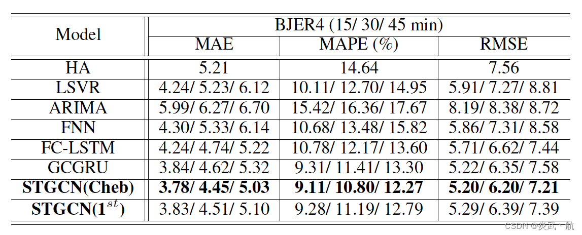
Table 1: Performance comparison of different approaches on the dataset BJER4.
表1: 数据集BJER4上不同方法的性能比较。

Table 2: Performance comparison of different approaches on the dataset PeMSD7.
表2: 不同方法在数据集PeMSD7上的性能比较。
Benefits of Spatial Topology(空间拓扑的优势)
Previous methods did not incorporate spatial topology and modeled the time series in a coarse-grained way. Differently, through modeling spatial topology of the sensors, our model STGCN has achieved a significant improvement on short and mid-and-long term forecasting. The advantage of STGCN is more obvious on dataset PeMSD7 than BJER4, since the sensor network of PeMS is more complicated and structured (as illustrated in Figure 3), and our model can effectively utilize spatial structure to make more accurate predictions.
以前的方法没有结合空间拓扑,也没有以粗粒度的方式对时间序列建模。不同的是,通过对传感器空间拓扑的建模,我们的模型STGCN在短期和中期预测方面取得了显著的改进。STGCN在数据集PeMSD7上的优势比BJER4更明显,因为PeMS的传感器网络更复杂、更结构化(如图3所示),我们的模型可以有效地利用空间结构进行更准确的预测。
To compare three methods based on graph convolution: GCGRU, STGCN(Cheb) and STGCN( 1 s t 1^{st} 1st), we show their predictions during morning peak and evening rush hours, as shown in Figure 4. It is easy to observe that our proposal STGCN captures the trend of rush hours more accurately than other methods; and it detects the ending of the rush hours earlier than others. Stemming from the efficient graph convolution and stacked temporal convolution structures, our model is capable of fast responding to the dynamic changes among the traffic network without over-reliance on historical average as most of recurrent networks do.
为了比较三种基于图卷积的方法:GCGRU, STGCN(Cheb)和STGCN( 1 s t 1^{st} 1st),我们展示了它们在早高峰和晚高峰时段的预测,如图4所示。不难看出,我们的建议STGCN比其他方法更准确地捕捉到高峰时间的趋势;它能比其他时间更早地检测到高峰时段的结束。基于高效的图卷积和叠加的时间卷积结构,我们的模型能够快速响应交通网络之间的动态变化,而不像大多数循环网络那样过度依赖历史平均。
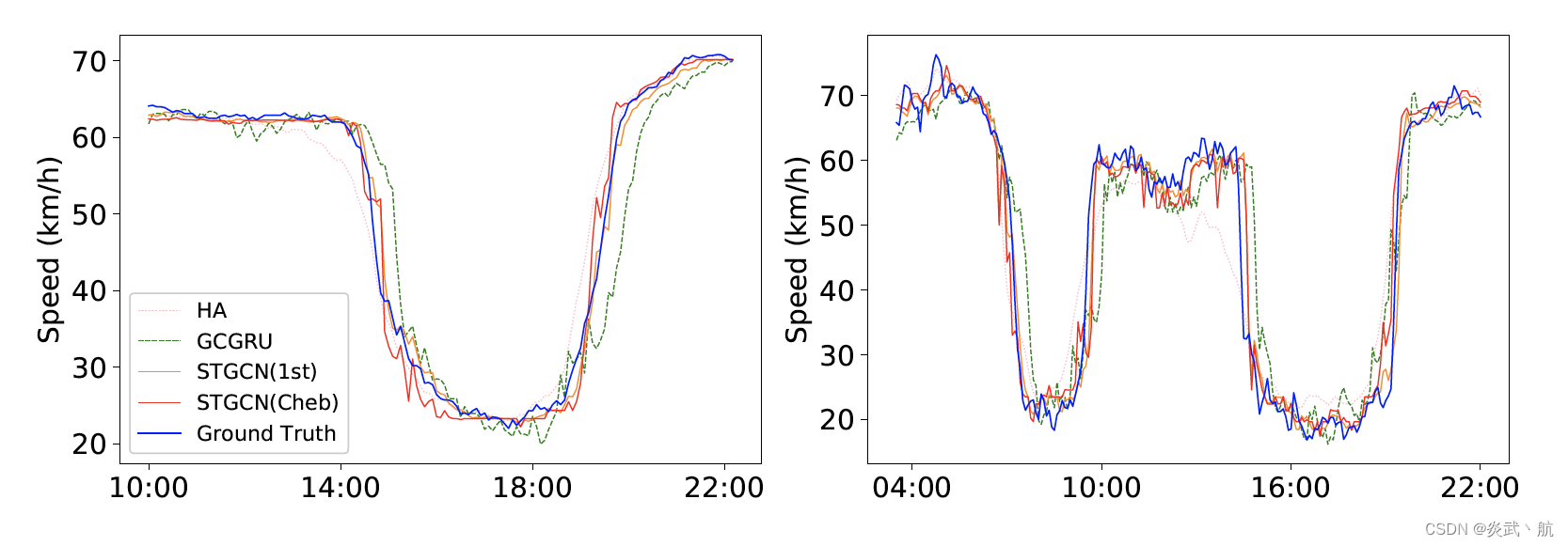
Figure 4: Speed prediction in the morning peak and evening rush hours of the dataset PeMSD7.
图4: 数据集PeMSD7早高峰和晚高峰速度预测
Training Efficiency and Generalization(训练效率与概括)
To see the benefits of the convolution along time axis in our proposal, we summarize the comparison of training time between STGCN and GCGRU in Table 3. In terms of fairness, GCGRU consists of three layers with 64 64 64, 64 64 64, 128 128 128 units respectively in the experiment for PeMSD7(M), and STGCN uses the default settings as described in Section 4.3. Our model STGCN only consumes 272 \bf272 272 seconds, while RNN-type of model GCGRU spends 3 , 824 \bf3, 824 3,824 seconds on PeMSD7(M). This 14 \bf14 14 times acceleration of training speed mainly benefits from applying the temporal convolution instead of recurrent structures, which can achieve fully parallel training rather than exclusively relying on chain structures as RNN do. For PeMSD7(L), GCGRU has to use the half of batch size since its GPU consumption exceeded the memory capacity of a single card (results marked as “ ∗ * ∗” in Table 2); while STGCN only need to double the channels in the middle of ST-Conv blocks. Even though our model still consumes less than a tenth of the training time of model GCGRU under this circumstance. Meanwhile, the advantages of the 1 s t 1^{st} 1st-order approximation have appeared since it is not restricted to the parameterization of polynomials. The model STGCN( 1 s t 1^{st} 1st) speeds up around 20 % 20\% 20% on a larger dataset with a satisfactory performance compared with STGCN(Cheb).
为了看到我们的方案中沿时间轴卷积的好处,我们在表3中总结了STGCN和GCGRU训练时间的比较。在公平性方面,在PeMSD7(M)实验中,GCGRU分为三层,分别为64,64,128个单元,STGCN采用4.3节的默认设置。我们的模型STGCN只消耗 272 \bf272 272 秒,而RNN型的模型GCGRU在PeMSD7(M)上花费 3 , 824 \bf3, 824 3,824 秒。这 14 \bf14 14 倍的训练速度的加速主要得益于使用时间卷积而不是循环结构,它可以实现完全的并行训练,而不是像RNN那样完全依赖于链结构。对于PeMSD7(L), GCGRU需要使用批大小的一半,因为它的GPU消耗超过了单个卡的内存容量(结果在表2中标记为“*”);而STGCN只需要将ST-Conv块中间的信道加倍即可。尽管在这种情况下,我们的模型所消耗的训练时间还不到模型GCGRU的十分之一。同时,由于不局限于多项式的参数化, 1 1 1 阶近似的优点也显现出来。与STGCN(Cheb)相比,模型STGCN( 1 s t 1^{st} 1st)在更大的数据集上加速约 20 % 20\% 20% ,性能令人满意。
In order to further investigate the performance of compared deep learning models, we plot the RMSE and MAE of the test set of PeMSD7(M) during the training process, see Figure 5. Those figures also suggest that our model can achieve much faster training procedure and easier convergences. Thanks to the special designs in ST-Conv blocks, our model has superior performances in balancing time consumption and parameter settings. Specifically, the number of parameters in STGCN ( 4.54 × 1 0 5 4.54×10^5 4.54×10⁵) only accounts for around two third of GCGRU, and saving over 95 % 95\% 95% parameters compared to FC-LSTM.
为了进一步研究比较的深度学习模型的性能,我们绘制了PeMSD7(M) 测试集在训练过程中的RMSE和MAE,见图5。这些数据还表明,我们的模型可以实现更快的训练过程和更容易的收敛。由于ST-Conv模块的特殊设计,我们的模型在平衡时间消耗和参数设置方面具有优越的性能。其中STGCN的参数数量 ( 4.54 × 1 0 5 4.54×10^5 4.54×10⁵) 仅占GCGRU的三分之二左右,比FC-LSTM节省了 95 % 95\% 95% 以上的参数。
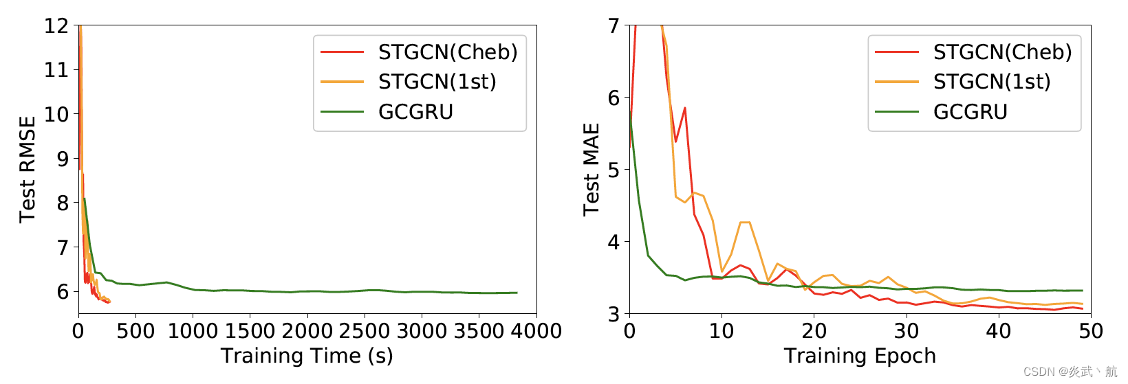
Figure 5: Test RMSE versus the training time (left); Test MAE versus the number of training epochs (right). (PeMSD7(M))
图5:测试RMSE与训练时间(左); 测试MAE与训练期的数量(右)。(PeMSD7 (M))
参考文献
[Chen et al., 2001] Chao Chen, Karl Petty, Alexander Skabardonis, Pravin Varaiya, and Zhanfeng Jia. Freeway performance measurement system: mining loop detector data. Transportation Research Record: Journal of the Transportation Research Board, (1748):96–102, 2001.
[Li et al., 2015] Yexin Li, Yu Zheng, Huichu Zhang, and Lei Chen. Traffic prediction in a bike-sharing system. In SIGSPATIAL, page 33. ACM, 2015.
[Sutskever et al., 2014] Ilya Sutskever, Oriol Vinyals, and Quoc V Le. Sequence to sequence learning with neural networks. In NIPS, pages 3104–3112, 2014.
[Li et al., 2018] Yaguang Li, Rose Yu, Cyrus Shahabi, and Yan Liu. Diffusion convolutional recurrent neural network: Data-driven traffic forecasting. In ICLR, 2018.