Code1:
filename = {str} 'tfidf_matrix'
filename = {str} 'tfidf_matrix'
tfidf = {ndarray: (15, 47)} [[0.         1.32827152 1.80872453 0.         0.         0.,  0.         0.         0.         0.         0.         1.45464719,  0.         0.         0.         0.         0.         0.,  0.         0.         0.         0.         1.60931851 0.,  1.8087
vocab = {list: 47} ['have', 'like', 'here', 'tree', 'morning', 'not', 'study', 'and', 'do', 'It', 'party', 'it', 'will', 'your', 'but', 'am', 'who', 'dog', 'care', 'today', 'that', 'bring', 'good', 'bob', 'to', 'cat', 'a', 'coffee', 'apple', 'be', 'there', 'time', 'is', 'cup
def show_tfidf(tfidf, vocab, filename):
# [n_doc, n_vocab]
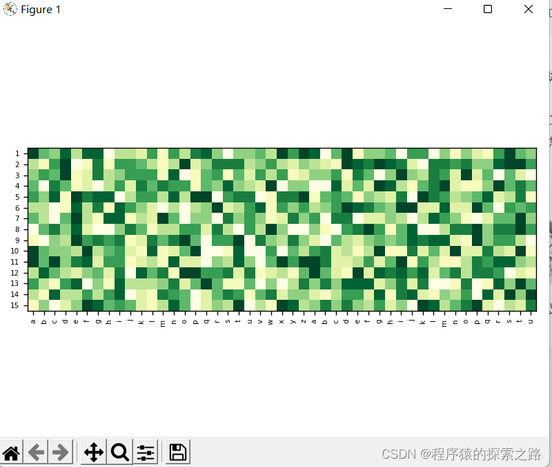
plt.imshow(tfidf, cmap="YlGn", vmin=tfidf.min(), vmax=tfidf.max())
plt.xticks(np.arange(tfidf.shape[1]), vocab, fontsize=6, rotation=90)
plt.yticks(np.arange(tfidf.shape[0]), np.arange(1, tfidf.shape[0]+1), fontsize=6)
plt.tight_layout()
# creating the output folder
output_folder = './visual/results/'
os.makedirs(output_folder, exist_ok=True)
plt.savefig(os.path.join(output_folder, '%s.png') % filename, format="png", dpi=500)
plt.show()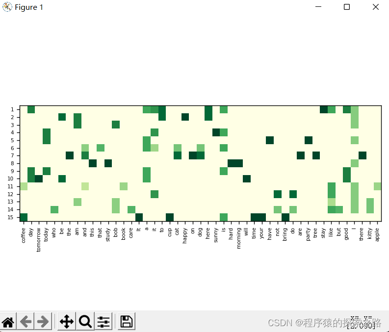
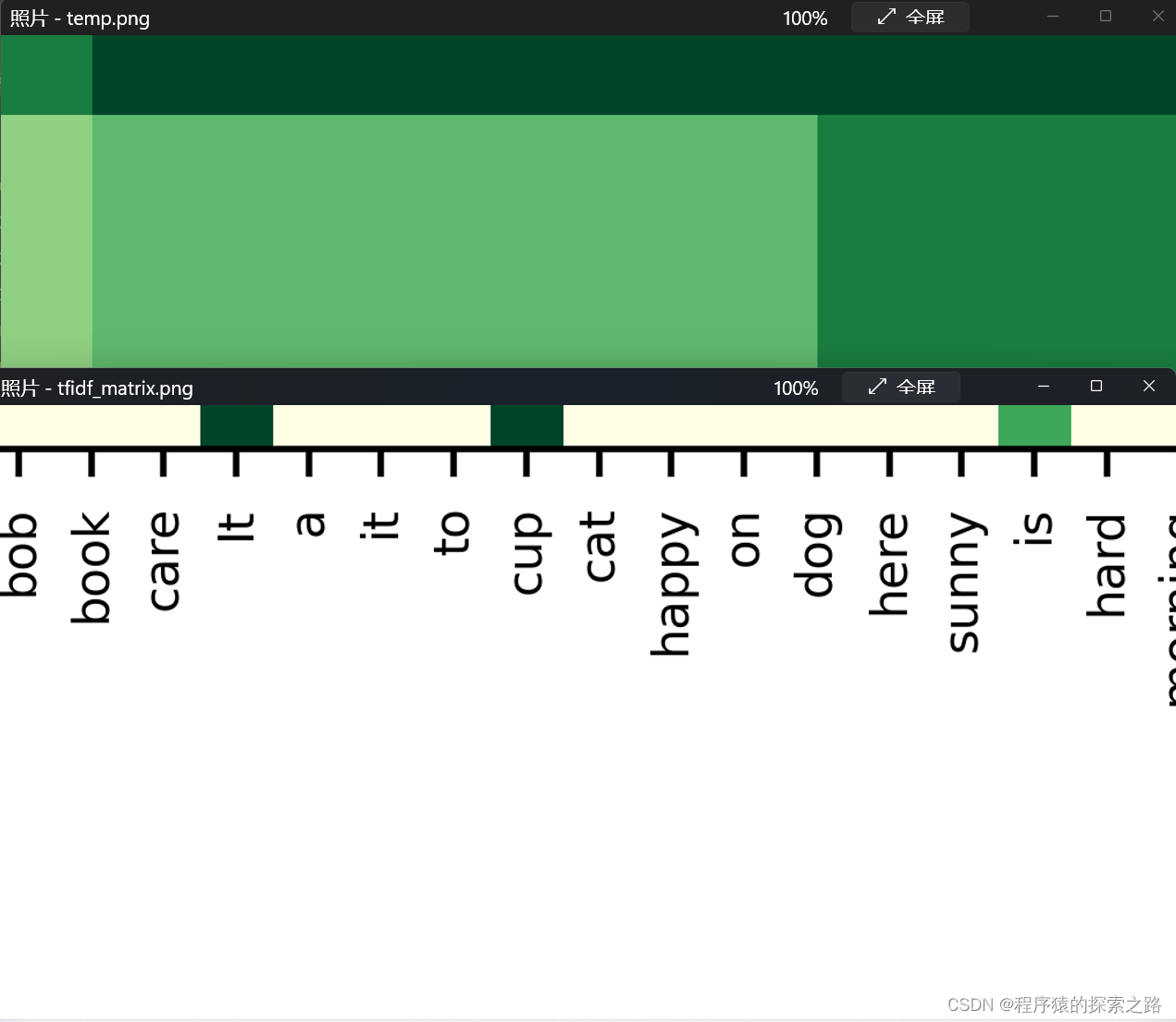
注1:比较 plt.savefig()参数中 dpi = 5000 和 dpi=500的区别:
上面的图片是dpi=5000的实际大小,下面的图片是dpi=500的实际大小,前者大小是后者的十倍。
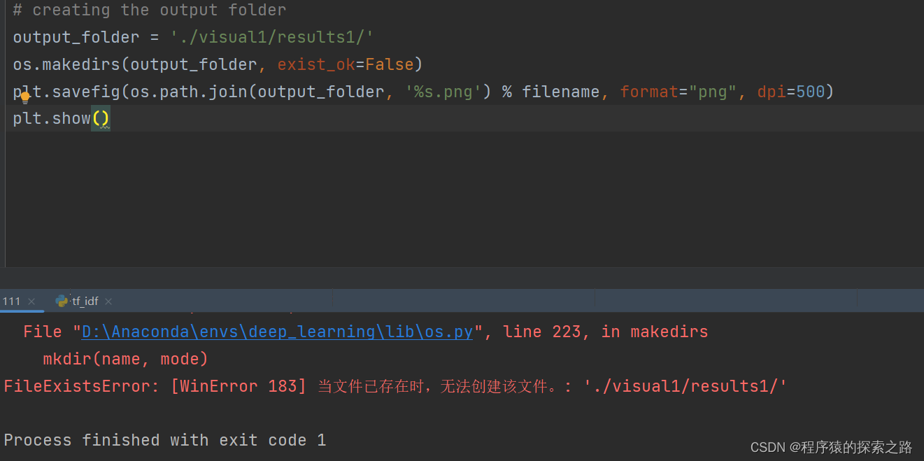
注2:os.makedirs()的参数exist_ok 设置为False,如果路径存在,则不能创建路径,并返回错误信息;将exist_ok设置为True,如果路径不存在,创建路径,如果存在则不再创建。
Code2:
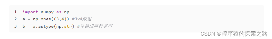
注:二维字符数组的一种实现方法。
import matplotlib.pyplot as plt
import numpy as np
import os


# tfidf=np.random.randint((15,47))
tfidf=np.random.randint(low=10,size=(15,47))
print(tfidf)
# input()
vocab=[]
print(type(vocab))
# 'x'-'a' % ('z'-'a'+1) +'a'
for i in range(47):
    if i<26:
        vocab.append(str(chr((ord('a')+i)%ord('a')+ord('a'))))
    else:
        i%=26
        vocab.append(str(chr((ord('a')+i)%ord('a')+ord('a'))))
filename="temp"
print(type(vocab[0]))
# vocab=np.array(vocab)
# vocab=vocab.reshape(vocab.shape[0],1).tolist()
# print(vocab.shape)
# print(type(vocab[0,0]))


# [n_doc, n_vocab]
plt.imshow(tfidf, cmap="YlGn", vmin=tfidf.min(), vmax=tfidf.max())
plt.xticks(np.arange(tfidf.shape[1]), vocab, fontsize=6, rotation=90)
plt.yticks(np.arange(tfidf.shape[0]), np.arange(1, tfidf.shape[0]+1), fontsize=6)
plt.tight_layout()
# creating the output folder
output_folder = './visual1/results1/'
os.makedirs(output_folder, exist_ok=True)
plt.savefig(os.path.join(output_folder, '%s.png') % filename, format="png", dpi=500)
plt.show()
D:\Anaconda\envs\deep_learning\python.exe C:/Users/王斌/NLP-Tutorials/111.py
[[9 5 4 8 3 8 8 0 3 3 2 6 1 6 3 7 8 4 0 4 4 5 3 9 6 9 8 0 5 9 1 4 4 5 0 6
6 0 4 1 4 2 1 6 9 5 4]
[3 1 6 9 0 1 7 1 6 6 5 3 1 3 9 2 4 7 7 7 3 4 6 3 2 4 3 2 1 9 8 7 9 8 7 2
0 7 7 6 7 4 4 8 9 9 6]
[4 6 5 9 1 2 7 3 4 6 6 6 1 8 0 1 5 6 1 5 2 6 3 6 1 2 4 4 6 1 7 5 0 4 9 4
3 7 6 2 9 2 5 0 5 2 0]
[5 0 7 5 1 2 0 3 6 2 7 5 7 6 6 1 5 4 8 4 3 2 9 0 4 4 0 0 8 2 5 2 9 8 3 1
5 7 9 2 1 1 4 9 5 7 5]
[6 4 8 1 9 7 8 8 0 3 6 6 3 8 3 9 9 0 6 7 7 0 1 7 7 9 1 5 6 5 1 4 3 2 7 0
9 7 6 3 4 5 8 2 3 7 1]
[3 3 0 1 8 3 7 1 8 6 4 2 0 3 0 3 4 9 2 3 6 8 1 6 4 6 3 4 6 9 8 7 5 4 9 9
2 2 8 2 2 9 5 0 6 5 6]
[5 3 0 5 9 3 1 8 8 1 3 2 9 5 0 4 4 0 7 4 6 4 1 2 7 4 6 0 7 7 0 2 2 4 3 0
3 8 6 4 1 0 2 5 5 9 4]
[0 5 7 4 8 2 0 0 4 7 5 1 3 3 6 6 2 7 3 0 6 3 9 4 0 0 4 1 0 6 7 9 6 1 5 8
0 0 3 7 7 9 4 7 7 9 6]
[1 0 4 3 9 6 7 6 7 1 2 7 5 7 9 5 0 6 6 9 0 7 4 3 7 4 2 0 5 3 2 4 5 4 5 8
7 8 8 2 1 9 4 6 6 3 0]
[9 5 4 4 3 9 3 5 6 2 1 8 1 2 5 9 0 0 1 8 0 0 6 0 5 3 6 7 2 3 1 3 9 1 1 7
2 5 2 9 2 2 7 3 2 9 1]
[9 5 9 4 7 8 2 6 6 1 2 3 1 8 2 2 0 4 3 8 4 0 5 9 6 9 9 7 2 2 3 6 2 5 9 1
6 3 1 1 3 7 6 8 8 4 3]
[3 8 5 3 2 4 5 2 7 0 8 5 7 1 9 9 6 6 7 2 7 1 2 3 1 5 9 5 2 1 9 2 8 7 8 6
8 2 5 7 3 7 7 6 0 2 1]
[6 3 1 6 8 0 4 1 8 3 3 3 4 7 2 5 9 5 1 1 5 0 4 0 3 7 4 7 4 8 8 8 2 4 7 2
7 0 0 1 7 0 1 8 4 9 5]
[3 1 8 3 3 6 3 6 8 0 2 1 7 6 5 0 2 5 7 6 1 5 7 2 4 4 2 1 3 6 6 2 8 1 7 8
2 1 4 3 6 0 8 2 9 4 9]
[1 4 0 2 4 9 8 5 6 5 2 1 3 8 5 0 2 4 3 9 0 3 1 9 8 3 4 7 4 7 4 3 6 2 4 0
9 8 3 5 7 9 2 0 3 2 7]]
<class 'list'>
<class 'str'>
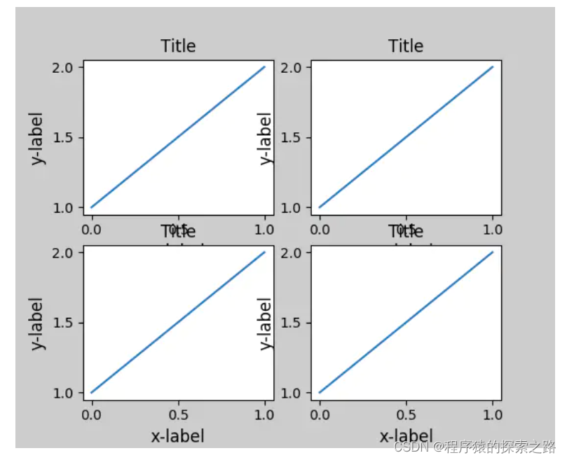
1. tight_layout()

使用前:
使用后: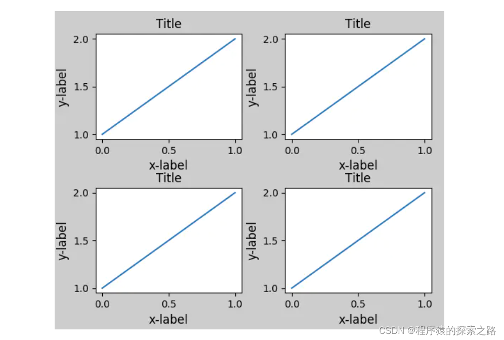
refer: Matplotlib 中文用户指南 3.4 密致布局指南 - 简书
2. plt.xticks()


refer: plt.xticks()_SilenceHell的博客-CSDN博客_plt.xticks
3. plt.savefig()
注:

正文: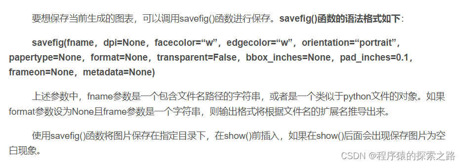
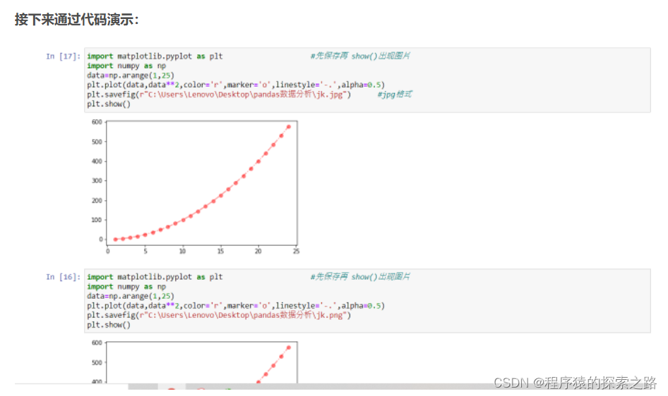
import matplotlib.pyplot as plt #先保存再 show()出现图片
import numpy as np
data=np.arange(1,25)
plt.plot(data,data**2,color='r',marker='o',linestyle='-.',alpha=0.5)
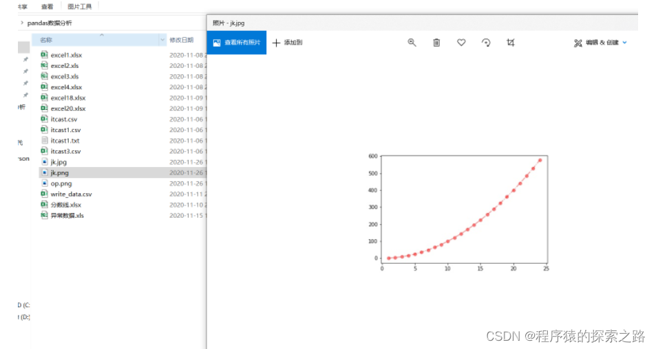
plt.savefig(r"C:\Users\Lenovo\Desktop\pandas数据分析\jk.jpg") #jpg格式
plt.show()
import matplotlib.pyplot as plt #先保存再 show()出现图片
import numpy as np
data=np.arange(1,25)
plt.plot(data,data**2,color='r',marker='o',linestyle='-.',alpha=0.5)
plt.savefig(r"C:\Users\Lenovo\Desktop\pandas数据分析\jk.png")
plt.show()
#先show()再保存
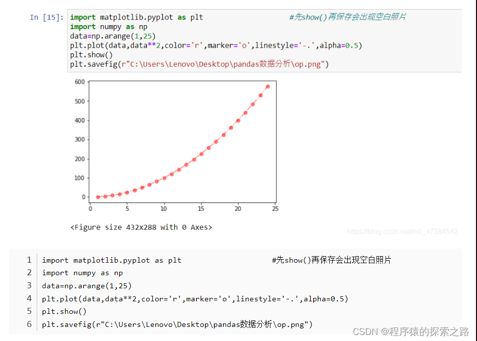

refer: Matplotlib本地保存图形—savefig()方法_KJ.JK的博客-CSDN博客_savefig
4. plt.imshow()
imshow:热图(heatmap)是数据分析的常用方法,通过色差、亮度来展示数据的差异、易于理解。Python在Matplotlib库中,调用imshow()函数实现热图绘制。
plt.imshow(
    X,
    cmap=None,
    norm=None,
    aspect=None,
    interpolation=None,
    alpha=None,
    vmin=None,
    vmax=None,
    origin=None,
    extent=None,
    shape=None,
    filternorm=1,
    filterrad=4.0,
    imlim=None,
    resample=None,
    url=None,
    *,
    data=None,
    **kwargs,
)
**X:**
图像数据。支持的数组形状是:
(M,N) :带有标量数据的图像。数据可视化使用色彩图。
(M,N,3) :具有RGB值的图像(float或uint8)。
(M,N,4) :具有RGBA值的图像(float或uint8),即包括透明度。
前两个维度(M,N)定义了行和列图片,即图片的高和宽;
RGB(A)值应该在浮点数[0, ..., 1]的范围内,或者
整数[0, ... ,255]。超出范围的值将被剪切为这些界限。
**cmap:**
将标量数据映射到色彩图
颜色默认为:rc:image.cmap。
**norm :**
~matplotlib.colors.Normalize
如果使用scalar data ,则Normalize会对其进行缩放[0,1]的数据值内。
默认情况下,数据范围使用线性缩放映射到颜色条范围。 RGB(A)数据忽略该参数。
**aspect:**
{'equal','auto'}或float,可选
控制轴的纵横比。该参数可能使图像失真,即像素不是方形的。
equal:确保宽高比为1,像素将为正方形。(除非像素大小明确地在数据中变为非正方形,坐标使用 extent )。
auto: 更改图像宽高比以匹配轴的宽高比。通常,这将导致非方形像素。
**interpolation:**
str
使用的插值方法
支持的值有:'none', 'nearest', 'bilinear', 'bicubic','spline16', 'spline36', 'hanning', 'hamming', 'hermite', 'kaiser',
'quadric', 'catrom', 'gaussian', 'bessel', 'mitchell', 'sinc','lanczos'.
如果interpolation = 'none',则不执行插值
**alpha:**
alpha值,介于0(透明)和1(不透明)之间。RGBA输入数据忽略此参数。
**vmin, vmax : scalar,**
如果使用* norm 参数,则忽略 vmin , vmax *。
vmin,vmax与norm结合使用以标准化亮度数据。
**origin : {'upper', 'lower'}**
将数组的[0,0]索引放在轴的左上角或左下角。
'upper'通常用于矩阵和图像。
请注意,垂直轴向上指向“下”但向下指向“上”。
**extent:(left, right, bottom, top)**
数据坐标中左下角和右上角的位置。 如果为“无”,则定位图像使得像素中心落在基于零的(行,列)索引上。