Global Filter Networks for Image Classification

[pdf] [project] [github]

Abstract

1 Introduction

2.1 Vision transformers

2.2 MLP-like models

2.3 Applications of Fourier transform in vision

3 Method

3.1 Preliminaries: discrete Fourier transform

3.2 Global Filter Networks

4 Experiments

4.3 Analysis and visualization

Appendix

B Implementation Details

Abstract

Recent advances in self-attention and pure multi-layer perceptrons (MLP) models for vision have shown great potential in achieving promising performance with fewer inductive biases. These models are generally based on learning interaction among spatial locations from raw data. The complexity of self-attention and MLP grows quadratically as the image size increases, which makes these models hard to scale up when high-resolution features are required.

In this paper, we present the Global Filter Network (GFNet), a conceptually simple yet computationally efficient architecture, that learns long-term spatial dependencies in the frequency domain with log-linear complexity. Our architecture replaces the self-attention layer in vision transformers with three key operations: a 2D discrete Fourier transform, an element-wise multiplication between frequency-domain features and learnable global filters, and a 2D inverse Fourier transform.

We exhibit favorable accuracy/complexity trade-offs of our models on both ImageNet and downstream tasks. Our results demonstrate that GFNet can be a very competitive alternative to transformer-style models and CNNs in efficiency, generalization ability and robustness.

研究背景和动机：

视觉的 self-attention (ViT) 和纯多层感知器 (MLP) 模型的最新进展显示了在较少归纳偏差的情况下实现有前景的性能的巨大潜力。这些模型通常基于从原始数据中学习空间位置之间的相互作用。随着图像尺寸的增加，self-attention 和 MLP 的复杂性呈二次增长，这使得这些模型在需要高分辨率特性时很难扩大。

研究内容：

本文提出了全局滤波网络 (GFNet)，一个概念简单但计算效率高的架构，它学习在频率域具有对数线性复杂度的长距离空间依赖关系。本文的架构用三个关键操作取代了 ViT 中的 self-attention：一个 2D 离散傅里叶变换，一个频域特征和可学习的全局滤波器之间的元素乘法，和一个 2D 傅里叶反变换。

研究结论：

本文的模型在 ImageNet 和下游任务上都表现出了良好的准确性和复杂性。结果表明，GFNet 在效率、泛化能力和鲁棒性方面可以成为 transformer 式模型和 CNN 非常有竞争力的替代。

1 Introduction

The transformer architecture, originally designed for the natural language processing (NLP) tasks [43], has shown promising performance on various vision problems recently [9, 40, 27, 49, 4]. Different from convolutional neural networks (CNNs), vision transformer models use self-attention layers to capture long-term dependencies, which are able to learn more diverse interactions between spatial locations. The pure multi-layer perceptrons (MLP) models [38, 39] further simplify the vision transformers by replacing the self-attention layers with MLPs that are applied across spatial locations. Since fewer inductive biases are introduced, these two kinds of models have the potential to learn more generic and flexible interactions among spatial locations from raw data.

Transformer 架构最初是为自然语言处理 (NLP) 任务设计的，最近在各种视觉问题上显示出了良好的性能。与卷积神经网络 (CNN) 不同，vision transformer 模型使用 self-attention 层来捕捉长距离依赖关系，能够了解空间位置之间更多样化的交互。纯多层感知器 (MLP) 模型通过用应用于空间位置的 MLP 替换 self-attention 层，进一步简化了 vision transformer。由于引入的归纳偏差较少，这两种模型有可能从原始数据中了解更多的一般和灵活的空间位置之间的相互作用。

One primary challenge of applying self-attention and pure MLP models to vision tasks is the considerable computational complexity that grows quadratically as the number of tokens increases. Therefore, typical vision transformer style models usually consider a relatively small resolution for the intermediate features (e.g. 14 × 14 tokens are extracted from the input images in both ViT [9] and MLP-Mixer [38]). This design may limit the applications of downstream dense prediction tasks like detection and segmentation. A possible solution is to replace the global self-attention with several local self-attention like Swin transformer [27]. Despite the effectiveness in practice, local self-attention brings quite a few hand-made choices (e.g., window size, padding strategy, etc.) and limits the receptive field of each layer.

将 self-attention 和纯 MLP 模型应用于视觉任务的一个主要挑战是巨大的计算复杂性，随着 tokens 数量的增加而二次方增长。因此，典型的 vision transformer 风格的模型通常考虑中间特征的相对较小的分辨率 (例如，从ViT [9] 和 MLP-Mixer [38] 的输入图像中提取 14 × 14 tokens)。这种设计可能会限制检测和分割等下游密集预测任务的应用。一个可能的解决方案是用几个局部的 self-attention 来替代全局的 self-attention，比如 Swin transformer [27]。尽管在实践中有效，局部的 self-attention 带来了相当多的人工选择 (例如，窗口大小，填充策略等)，并限制了每个层的接受域。

In this paper, we present a new conceptually simple yet computationally efficient architecture called Global Filter Network (GFNet), which follows the trend of removing inductive biases from vision models while enjoying the log-linear complexity in computation.

The basic idea behind our architecture is to learn the interactions among spatial locations in the frequency domain.

Different from the self-attention mechanism in vision transformers and the fully connected layers in MLP models, the interactions among tokens are modeled as a set of learnable global filters that are applied to the spectrum of the input features.

Since the global filters are able to cover all the frequencies, our model can capture both long-term and short-term interactions.

The filters are directly learned from the raw data without introducing human priors.

Our architecture is largely based on the vision transformers only with some minimal modifications. We replace the self-attention sub-layer in vision transformers with three key operations: a 2D discrete Fourier transform to convert the input spatial features to the frequency domain, an element-wise multiplication between frequency-domain features and the global filters, and a 2D inverse Fourier transform to map the features back to the spatial domain.

Since the Fourier transform is used to mix the information of different tokens, the global filter is much more efficient compared to the self-attention and MLP thanks to the O(Llog L) complexity of the fast Fourier transform algorithm (FFT) [6].

Benefiting from this, the proposed global filter layer is less sensitive to the token length L and thus is compatible with larger feature maps and CNN-style hierarchical architectures without modifications.

The overall architecture of GFNet is illustrated in Figure 1. We also compare our global filter with prevalent operations in deep vision models in Table 1.

本段系统介绍了 GFNet：

本文提出了一种新的概念简单但计算效率高的架构，称为全局滤波网络 (GFNet)，它遵循了消除视觉模型归纳偏差的趋势，同时享受了对数线性计算的复杂性。

该架构的基本思想是了解频率域中空间位置之间的相互作用。

不同于 vision transformer 中的 self-attention 机制和 MLP 模型中的全连接层，tokens 之间的交互被建模为一组可学习的全局滤波器，应用于输入特征的频谱。

由于全局滤波器能够覆盖所有频率，本文的模型可以捕捉长期和短期的交互作用。

滤波器是直接从原始数据学习，而不引入人为先验。

本文的架构很大程度上是基于 vision transformer，只是做了一些最小的修改。本文采用三个关键操作来替换 vision transformer 中的 self-attention 层：二维离散傅里叶变换将输入空间特征转换为频域，在频域特征和全局滤波器之间进行元素乘法，以及二维反傅里叶变换将特征映射回空间域。

由于傅里叶变换用于混合不同 tokens 的信息，由于快速傅里叶变换算法 (FFT) 的 O(Llog L) 复杂度，全局滤波器比 self-attention 和 MLP 更有效。因此，所提出的全局滤波层对 token 长度 L 的敏感性较低，因此无需修改即可兼容更大的特征映射和 CNN 风格的层次结构。

GFNet 的总体架构如图 1 所示。表 1 中，全局滤波器与深度视觉模型中的普遍操作进行了比较。

Our experiments on ImageNet verify the effectiveness of GFNet. With a similar architecture, our model outperform the recent vision transformer and MLP models including DeiT [40], ResMLP [39] and gMLP [26]. When using the hierarchical architecture, GFNet can further enlarge the gap. GFNet also works well on downstream transfer learning and semantic segmentation tasks. Our results demonstrate that GFNet can be a very competitive alternative to transformer-style models and CNNs in efficiency, generalization ability and robustness.

在 ImageNet 上的实验验证了 GFNet 的有效性。使用类似的架构，本文的模型优于最近的 ViT 和MLP 模型，包括 DeiT、ResMLP 和 gMLP。当使用层次结构时，GFNet 可以进一步扩大差距。GFNet 在下游迁移学习和语义分割任务上也很有效。结果表明，GFNet 在效率、泛化能力和鲁棒性方面可以成为 transformer 式模型和 CNN 非常有竞争力的替代品。

2.1 Vision transformers

Since Dosovitskiy et al. [9] introduce transformers to the image classification and achieve a competitive performance compared to CNNs, transformers begin to exhibit their potential in various vision tasks [3, 4, 49]. Recently, there are a large number of works which aim to improve the transformers [40, 41, 27, 45, 18, 10, 48]. These works either seek for better training strategies [40, 10] or design better architectures [27, 45, 48] or both [41, 10]. However, most of the architecture modification of the transformers [45, 18, 27, 48] introduces additional inductive biases similar to CNNs. In this work, we only focus on the standard transformer architecture [9, 40] and our goal is to replace the heavy self-attention layer ( $\mathcal{O}(L ^2 )$ ) to an more efficient operation which can still model the interactions among different spatial locations without introducing the inductive biases associated with CNNs.

由于Dosovitskiy et al. 将 transformer 引入到图像分类中，并取得了与 CNN 相媲美的性能，transformer 开始在各种视觉任务中发挥其潜力。最近，有大量的工作旨在改进 transformer。这些作品要么寻求更好的培训策略，要么设计更好的架构，要么两者兼得。然而，大多数 transformer 的结构修改引入了类似 CNN 的额外归纳偏差。本文只关注标准的 transformer 架构，目标是将 heavy self-attention layer ( $\mathcal{O}(L ^2 )$ ) 替换为更有效的操作，该操作仍然可以模拟不同空间位置之间的相互作用，而不会引入与 CNN 相关的归纳偏差。

[40] Hugo Touvron, Matthieu Cord, Matthijs Douze, Francisco Massa, Alexandre Sablayrolles, and Hervé Jégou. Training data-efficient image transformers & distillation through attention. arXiv preprint arXiv:2012.12877, 2020.

[10] Chengyue Gong, Dilin Wang, Meng Li, Vikas Chandra, and Qiang Liu. Improve vision transformers training by suppressing over-smoothing. arXiv preprint arXiv:2104.12753, 2021.

[27] Ze Liu, Yutong Lin, Yue Cao, Han Hu, Yixuan Wei, Zheng Zhang, Stephen Lin, and Baining Guo. Swin transformer: Hierarchical vision transformer using shifted windows. arXiv preprint arXiv:2103.14030, 2021.

[45] Haiping Wu, Bin Xiao, Noel Codella, Mengchen Liu, Xiyang Dai, Lu Yuan, and Lei Zhang. Cvt: Introducing convolutions to vision transformers. arXiv preprint arXiv:2103.15808, 2021.

[48] Li Yuan, Yunpeng Chen, Tao Wang, Weihao Yu, Yujun Shi, Zihang Jiang, Francis EH Tay, Jiashi Feng, and Shuicheng Yan. Tokens-to-token vit: Training vision transformers from scratch on imagenet. arXiv preprint arXiv:2101.11986, 2021.

[41] Hugo Touvron, Matthieu Cord, Alexandre Sablayrolles, Gabriel Synnaeve, and Hervé Jégou. Going deeper with image transformers. arXiv preprint arXiv:2103.17239, 2021.

2.2 MLP-like models

More recently, there are several works that question the importance of self-attention in the vision transformers and propose to use MLP to replace the self-attention layer in the transformers [38, 39, 26]. The MLP-Mixer [38] employs MLPs to perform token mixing and channel mixing alternatively in each block. ResMLP [39] adopts a similar idea but substitutes the Layer Normalization with an Affine transformation for acceleration. The recently proposed gMLP [26] uses a spatial gating unit to re-weight tokens in the spatial dimension. However, all of the above models include MLPs to mix the tokens spatially, which brings two drawbacks: (1) like the self-attention in the transformers, the spatial MLP still requires computational complexity quadratic to the length of tokens. (2) unlike transformers, MLP models are hard to scale up to higher resolution since the weights of the spatial MLPs have fixed sizes. Our work follows this trend and successfully resolves the above issues in MLP-like models. The proposed GFNet enjoys log-linear complexity and can be easily scaled up to any resolution.

最近，有几篇文章质疑 vision transformers 中 self-attention 的重要性，并提出使用 MLP 来替代 transformer 中的 self-attention。MLP-Mixer [38] 使用 MLP 在每个块中交替地执行 tokens 混合和通道混合。ResMLP 采用了类似的思想，但是用仿射变换代替了层归一化来代替加速。最近提出的 gMLP 使用一个空间门控单元在空间维度上重新加权 。然而，上述所有模型都包含了 MLP 来在空间上混合 tokens，这带来了两个缺点: (1) 与 transformers 中的 self-attention 一样，空间 MLP 仍然需要 token 长度二次方的计算复杂度。(2) 与 transformers 不同，由于空间 MLP 的权重有固定的大小，因此 MLP 模型很难扩大到更高的分辨率。本文的工作遵循这一趋势，并成功地解决了上述问题在类 MLP 模型。GFNet 具有对数线性复杂度，可以很容易地扩展到任何分辨率。

MLP-Mixer: An all-MLP Architecture for Vision [2021]

ResMLP: Feedforward networks for image classification with data-efficient training [2021]

gMLP: Pay Attention to MLPs [2021]

2.3 Applications of Fourier transform in vision

Fourier transform has been an important tool in digital image processing for decades [33, 1]. With the breakthroughs of CNNs in vision [13, 12], there are a variety of works that start to incorporate Fourier transform in some deep learning method [25, 47, 8, 23]. Some of these works employ discrete Fourier transform to convert the images to the frequency domain and leverage the frequency information to improve the performance in certain tasks [23, 47], while others utilize the convolution theorem to accelerate the CNNs via fast Fourier transform (FFT) [25, 8]. In this work, we propose to use learnable filters to interchange information among the tokens in the Fourier domain, inspired by the frequency filters in the digital image processing [33]. We also take advantage of some properties of FFT to reduce the computational costs and the number of parameters.

傅里叶变换一直是数字图像处理的重要工具。随着 CNN 在视觉上的突破，有很多工作开始在一些深度学习方法中加入傅里叶变换。其中一些工作采用离散傅里叶变换将图像转换到频域，利用频率信息提高某些任务的性能，而另一些工作则利用卷积定理通过快速傅里叶变换 (FFT) 来加速 CNN。本工作中提出使用可学习滤波器来交换傅里叶域的 tokens 之间的信息，灵感来自于数字图像处理中的频率滤波器。本文还利用了 FFT 的一些性质，以减少计算成本和参数的数量。

3 Method

3.1 Preliminaries: discrete Fourier transform

We start by introducing the discrete Fourier transform (DFT), which plays an important role in the area of digital signal processing and is a crucial component in our GFNet. For clarity, We first consider the 1D DFT. Given a sequence of N complex numbers x[n], 0 ≤ n ≤ N − 1, the 1D DFT converts the sequence into the frequency domain by:

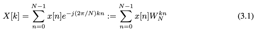
where j is the imaginary unit and $W_N = e^{-j(2\pi /N)}$ . The formulation of DFT in Equation (3.1) can be derived from the Fourier transform for continuous signal by sampling in both the time domain and the frequency domain (see Appendix A for details). Since X[k] repeats on intervals of length N, it is suffice to take the value of X[k] at N consecutive points k = 0, 1, . . . , N − 1. Specifically, X[k] represents to the spectrum of the sequence x[n] at the frequency $\omega _k = 2\pi k/N$ .

首先介绍离散傅里叶变换 (DFT)，它在数字信号处理领域发挥着重要作用，是 GFNet 的一个重要组成部分。为了清晰起见，首先考虑一维 DFT。给定一个包含 N 个复数的序列 x[n]， 0 ≤ n ≤ N−1,1D DFT 通过 (3.1) 将该序列转换为频域。其中 j 为虚单位， $W_N = e^{-j(2\pi /N)}$ 。对连续信号进行时域和频域采样的傅里叶变换，可推导出式 (3.1) 中 DFT 的表达式 (详见附录A)。由于 X[k] 在长度为 N 的间隔上重复，取 X[k] 在 N 个连续点 k = 0,1，…， n−1。具体来说，X[k] 表示序列 X[n] 在频率 $\omega _k = 2\pi k/N$ 处的频谱。

It is also worth noting that DFT is a one-to-one transformation. Given the DFT X[k], we can recover the original signal x[n] by the inverse DFT (IDFT):

For real input x[n], it can be proved that (see Appendix A) its DFT is conjugate symmetric, i.e., X[N − k] = X∗ [k]. The reverse is true as well: if we perform IDFT to X[k] which is conjugate symmetric, a real discrete signal can be recovered. This property implies that the half of the DFT $\{X[k] : 0 \leq k \leq \left \lceil N/2 \right \rceil\}$ contains the full information about the frequency characteristics of x[n].

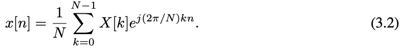
同样值得注意的是DFT是一个一对一的变换。给定 DFT X[k]，我们可以通过 (3.2) 式的逆 DFT (IDFT) 恢复原始信号 X[n]。

对于实输入 x[n]，可以证明 (见附录A) 其 DFT 是共轭对称的，即 x[n−k] = x∗[k]。反之亦然：如果对共轭对称的 X[k] 执行 IDFT，就可以恢复一个真实的离散信号。该性质表明 DFT $\{X[k] : 0 \leq k \leq \left \lceil N/2 \right \rceil\}$ 的一半包含 X[n] 频率特性的全部信息。

DFT is widely used in modern signal processing algorithms for mainly two reasons: (1) the input and output of DFT are both discrete thus can be easily processed by computers; (2) there exist efficient algorithms for computing the DFT. The fast Fourier transform (FFT) algorithms take advantage of the symmetry and periodicity properties of $W^{kn}_N$ and reduce the complexity to compute DFT from $\mathcal{O}(N^2 )$ to $\mathcal{O}(N log N)$ . The inverse DFT (3.2), which has a similar form to the DFT, can also be computed efficiently using the inverse fast Fourier transform (IFFT).

DFT 在现代信号处理算法中得到广泛应用，主要有两个原因： (1) DFT 的输入和输出都是离散的，便于计算机处理；(2) 存在计算 DFT 的有效算法。快速傅里叶变换 (FFT) 算法利用对称性和周期性的性质 $W^{kn}_N$ 和减少 DFT 的计算复杂度，从 $\mathcal{O}(N^2 )$ to $\mathcal{O}(N log N)$ 。逆 DFT (3.2) 有一个类似的DFT 的形式，也可以计算有效使用快速傅里叶逆变换 (传输线)。

快速傅里叶变换和逆变换可以用下面代码实现：

# Algorithm 1 Pseudocode of Global Filter Layer.
# x: the token features, B x H x W x D (where N = H * W)
# K: the frequency-domain filter, H x W_hat x D (where W_hat = W // 2 + 1, see Section 3.2 for details)

X = rfft2(x, dim=(1, 2))
X_tilde = X * K
x = irfft2(X_tilde, dim=(1, 2))

#rfft2/irfft2: 2D FFT/IFFT for real signal

The DFT described above can be extend to 2D signals. Given the 2D signal X[m, n], 0 ≤ m ≤ M − 1, 0 ≤ n ≤ N − 1, the 2D DFT of x[m, n] is given by:

The 2D DFT can be viewed as performing 1D DFT on the two dimensions alternatively. Similar to 1D DFT, 2D DFT of real input x[m, n] satisfied the conjugate symmetry property X[M − u, N − v] = X∗ [u, v]. The FFT algorithms can also be applied to 2D DFT to improve computational efficiency.

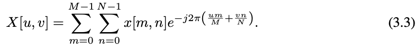
上述 DFT 可以推广到二维信号。给定二维信号 X[m, n]， 0 ≤ m ≤m−1,0 ≤ n ≤ n−1，X[m, n] 的二维 DFT 为 (3.3)。

二维 DFT 可以看作是在二维上进行一维 DFT。与一维 DFT 类似，实输入 x[m, n] 的 2D DFT 满足共轭对称性质 x[m−u, n−v] = x∗[u, v]。FFT 算法也可以应用于二维 DFT 中，以提高计算效率。

3.2 Global Filter Networks

Overall architecture

Recent advances in vision transformers [9, 40] demonstrate that models based on self-attention can achieve competitive performance even without the inductive biases associated with the convolutions. Henceforth, there are several works [39, 38] that exploit approaches (e.g., MLPs) other than self-attention to mix the information among the tokens. The proposed Global Filter Networks (GFNet) follows this line of work and aims to replace the heavy self-attention layer ( $\mathcal{O}(N^2 )$ ) with a simpler and more efficient one.

总体的结构

vision transformers 的最新进展表明，即使没有与卷积相关的归纳偏差，基于 self-attention 的模型也能实现 competitive 性能。因此，有几个工作利用除 self-attention 之外的方法 (如 MLP) 在 tokens 之间混合信息。本文的全局滤波网络 (GFNet) 遵循这一工作路线，旨在用一个更简单、更有效的层取代 heavy self-attention 层 ( $\mathcal{O}(N^2 )$ )。

The overall architecture of our model is depicted in Figure 1. Our model takes as an input H × W non-overlapping patches and projects the flattened patches into L = HW tokens with dimension D. The basic building block of GFNet consists of: 1) a global filter layer that can exchange spatial information efficiently ( $\mathcal{O}(L \log L)$ ); 2) a feedforward network (FFN) as in [9, 40]. The output tokens of the last block are fed into a global average pooling layer followed by a linear classifier.

模型的总体架构如图 1 所示。该模型以 H × W 非重叠斑块作为输入，将平坦斑块投射到 L = HW 的 D 维 tokens 中。GFNet 的基本构建模块包括：1) 一个能够有效交换空间信息的全局滤波层( $\mathcal{O}(L \log L)$ )；2) 前馈网络 (FFN)。最后一个块的输出 tokens 被输入到一个全局平均池化层，然后是一个线性分类器。

Global filter layer

We propose global filter layer as an alternative to the self-attention layer which can mix tokens representing different spatial locations. Given the tokens $x \in \mathbb{R}^{ H\times W\times D}$ , we first perform 2D FFT (see Section 3.1) along the spatial dimensions to convert x to the frequency domain:

where F[·] denotes the 2D FFT. Note that X is a complex tensor and represents the spectrum of x. We can then modulate the spectrum by multiplying a learnable filter $K \in \mathbb{C}^{ H\times W\times D}$ to the X:

where $\odot$ is the element-wise multiplication (also known as the Hadamard product). The filter K is called the global filter since it has the same dimension with X, which can represent an arbitrary filter in the frequency domain. Finally, we adopt the inverse FFT to transform the modulated spectrum $\tilde{X}$ back to the spatial domain and update the tokens:

本文提出全局滤波层作为 self-attention 层的替代方案，可以混合表示不同空间位置的符号。已知tokens $x \in \mathbb{R}^{ H\times W\times D}$ ，首先沿着空间维度进行 2D FFT (3.4)，将 x 转换为频域。式中 F[·] 为二维FFT。注意 X 是一个复张量，表示 x 的频谱。将一个可学习滤波器 $K \in \mathbb{C}^{ H\times W\times D}$ 乘以 X 来调制频谱，即公式 (3.5)。其中 $\odot$ 为元素乘法 (也称为 Hadamard 乘积)。滤波器 K 与 X 具有相同的维数，可以表示频域中的任意滤波器，因此称为全局滤波器。最后，采用逆 FFT 将已调制频谱 $\tilde{X}$ 归于空间域并更新 token，即 (3.6)。

The formulation of the global filter layer is motivated by the frequency filters in the digital image processing [33], where the global filter K can be regarded as a set of learnable frequency filters for different hidden dimensions. It can be proved (see Appendix A) that the global filter layer is equivalent to a depthwise global circular convolution with the filter size H × W. Therefore, the global filter layer is different from the standard convolutional layer which adopts a relatively small filter size to enforce the inductive biases of the locality. We also find although the proposed global filter can also be interpreted as a spatial domain operation, the filters learned in our networks exhibit more clear patterns in the frequency domain than the spatial domain, which indicates our models tend to capture relation in the frequency domain instead of spatial domain (see Figure 4). Note that the global filter implemented in the frequency domain is also much more efficient compared to the spatial domain, which enjoys a complexity of $\mathcal{O}(DL\log L)$ while the vanilla depthwise global circular convolution in the spatial domain has $\mathcal{O}(DL^2)$ complexity. We will also show that the global filter layer is better than its local convolution counterparts in the experiments.

全局滤波器层的公式是由数字图像处理中的频率滤波器提出的，其中全局滤波器 K 可以看作是一组具有不同隐藏维数的可学习频率滤波器。它可以证明 (见附件 A)，全局滤波层相当于尺寸为 H×W 的 depthwise 全局循环卷积滤波器。因此,，全局滤波器层不同于标准的卷积层采用一个相对较小的滤波器尺寸执行位置的 inductive biases。作者还发现，尽管提出的全局滤波器也可以解释为空间域操作，但网络中学习到的滤波器在频域比空间域表现出更清晰的模式，这表明 GFNet 模型倾向于在频域而不是空间域捕捉关系 (见图 4)。注意，在频域实现的全局滤波器也比空间域更有效，其复杂度为 $\mathcal{O}(DL\log L)$ ，而空间域 vanilla depthwise 全局深度循环卷积复杂度为 $\mathcal{O}(DL^2)$ 。本文还在实验中证明，全局滤波层比局部卷积层更好。

It is also worth noting that in the implementation, we make use of the property of DFT to reduce the redundant computation. Since x is a real tensor, its DFT X is conjugate symmetric, i.e. X[H − u, W − v, :] = X∗ [H, W, :]. Therefore, we can take only the half of the values in the X but preserve the full information at the same time:

Where $\mathcal{F}_r$ denotes the 2D FFT for real input. In this way, we can implement the global filter as $K_r \in \mathbb{C}^{ H\times \widehat{W}\times D}$ , which can reduce half the parameters. This can also ensure $\mathcal{F} ^{-1}_ r [K_r \odot X_r]$ is a real tensor, thus it can be added directly to the input x. The global filter layer can be easily in modern deep learning frameworks (e.g., PyTorch [32]), as is shown in Algorithm 1. The FFT and ITTF are well supported by GPU and CPU thanks to the acceleration libraries like ${\color{Orchid} \texttt{cuFFT}}$ and ${\color{Orchid} \texttt{mkl-fft}}$ , which makes our models perform well on hardware.

# Algorithm 1 Pseudocode of Global Filter Layer.
# x: the token features, B x H x W x D (where N = H * W)
# K: the frequency-domain filter, H x W_hat x D (where W_hat = W // 2 + 1, see Section 3.2 for details)

X = rfft2(x, dim=(1, 2))
X_tilde = X * K
x = irfft2(X_tilde, dim=(1, 2))

#rfft2/irfft2: 2D FFT/IFFT for real signal

另外值得注意的是，在实现模型时，利用了 DFT 的性质来减少冗余计算。由于 x 是一个实张量，其DFT x 是共轭对称的，即 x [H−u, W−v，:] = x∗[H, W，:]。因此，可以只取 X 中一半的值，同时保留完整的信息，如公式 (3.7)。其中 $\mathcal{F}_r$ 为实数输入的 2D FFT。这样，可以实现全局滤波器 $K_r \in \mathbb{C}^{ H\times \widehat{W}\times D}$ ，并减少一半的参数。这也可以确保 $\mathcal{F} ^{-1}_ r [K_r \odot X_r]$ 是一个实张量，因此它可以直接添加到输入 x 中。在现代深度学习框架 (如 PyTorch) 中，全局滤波层很容易实现，如算法 1 所示。由于 ${\color{Orchid} \texttt{cuFFT}}$ and ${\color{Orchid} \texttt{mkl-fft}}$ 等加速库，GPU 和 CPU 很好地支持 FFT 和 ITTF，这使得本文的模型在硬件上表现良好。

Relationship to other transformer-style models

The GFNet follows the line of research about the exploration of approaches to mix the tokens. Compared to existing architectures like vision transformers and pure MLP models, we exhibit that GFNet has several favorable properties:

1) GFNet is more efficient. The complexity of both the vision transformers [9, 40, 41] and the MLP models [38, 39] is $\mathcal{O}(L^2 )$ . Different from them, global filter layer only consists an FFT ( $\mathcal{O}(L\log L)$ ), an element-wise multiplication ( $\mathcal{O}(L)$ ) and an IFFT ( $\mathcal{O}(L)$ ), which means the total computational complexity is $\mathcal{O}(L\log L)$ .

2) Although pure MLP models are simpler compared to transformers, it is hard to fine-tune them on higher resolution (e.g., from 224 × 224 resolution to 384 × 384 resolution) since they can only process a fixed number of tokens. As opposed to pure MLP models, we will show that our GFNet can be easily scaled up to higher resolution. Our model is more flexible since both the FFT and the IFFT have no learnable parameters and can process sequences with arbitrary length. We can simply interpolate the global filter K to $K' \in\mathbb{ C} ^{H'\times W'\times D}$ for different inputs, where $H' \times W'$ is the target size. The interpolation is reasonable due to the property of DFT. Each element of the global filter K[u, v] corresponds to the spectrum of the filter at $\omega _u = 2\pi_u/H$ , $\omega _v = 2\pi_u/H$ and thus, the global filter K can be viewed as a sampling of a continuous spectrum $K(\omega _u, \omega _v)$ , where $\omega _u, \omega _v \in [0, 2\pi]$ . Hence, changing the resolution is equivalent to changing the sampling interval of $K(\omega _u, \omega _v)$ . Therefore, we only need to perform interpolation to shift from one resolution to another.

GFNet 遵循关于混合 tokens 方法探索的研究路线。与现有的 vision transformers 和pure MLP 模型相比，GFNet 具有以下几个优点：

1）GFNet更高效。vision transformers 和 MLP 模型的复杂度均为 $\mathcal{O}(L^2 )$ 。与它们不同的是，全局滤波层只包含一个 FFT ( $\mathcal{O}(L\log L)$ )，一个元素乘法 ( $\mathcal{O}(L)$ ) 和 IFFT ( $\mathcal{O}(L)$ )，这意味着总的计算复杂度是 $\mathcal{O}(L\log L)$ 。

2）GFNet 可以很容易地扩大到更高的分辨率，更加灵活。因为 FFT 和 IFFT 都没有可学习的参数，可以处理任意长度的序列。对于不同的输入，可以简单地将全局滤波器 K 插值到 $K' \in\mathbb{ C} ^{H'\times W'\times D}$ ，其中 $H' \times W'$ 为目标大小。由于 DFT 的特性，该插值方法是合理的。全局滤波器 K[u, v ] 的每个元素对应于滤波器在 $\omega _u = 2\pi_u/H$ ， $\omega _v = 2\pi_u/H$ 处的频谱，因此，全局滤波器 K 可以看作是连续频谱 $K(\omega _u, \omega _v)$ 的采样，其中 $\omega _u, \omega _v \in [0, 2\pi]$ 。因此，改变分辨率相当于改变 $K(\omega _u, \omega _v)$ 的采样间隔。因此，只需要执行插值来从一个分辨率转换到另一个分辨率。

We also notice recently a concurrent work FNet [24] leverages Fourier transform to mix tokens. Our work is distinct from FNet in three aspects: (1) FNet performs FFT to the input and directly adds the real part of the spectrum to the input tokens, which blends the information from different domains (spatial/frequency) together. On the other hand, GFNet draws motivation from the frequency filters, which is more reasonable. (2) FNet only keeps the real part of the spectrum. Note that the spectrum of real input is conjugate symmetric, which means the real part is exactly symmetric and thus contains redundant information. Our GFNet, however, utilizes this property to simplify the computation. (3) FNet is designed for NLP tasks, while our GFNet focuses on vision tasks. In our experiments, we also implement the FNet and show that our model outperforms it.

我们还注意到最近一个并行工作FNet[24]利用傅立叶变换来混合token。我们的工作与FNet有三个不同之处:(1)FNet对输入进行FFT，直接将频谱的实部加入到输入令牌中，将来自不同领域(空间/频率)的信息混合在一起。另一方面，GFNet从频率滤波器中提取动力，这更合理。(2) FNet只保留频谱的实部。注意实输入的频谱是共轭对称的，这意味着实部是完全对称的，因此包含冗余信息。然而，我们的GFNet利用这个属性来简化计算。(3) FNet是针对NLP任务设计的，而我们的GFNet专注于视觉任务。在我们的实验中，我们也实现了FNet，并表明我们的模型优于它。

Architecture variants

Due to the limitation from the quadratic complexity in the self-attention, vision transformers [9, 40] are usually designed to process a relatively small feature map (e.g., 14×14).

However, our GFNet, which enjoys log-linear complexity, avoids that problem. Since in our GFNet the computational costs do not grow such significantly when the feature map size increases, we can adopt a hierarchical architecture inspired by the success of CNNs [22, 13]. Generally speaking, we can start from a large feature map (e.g., 56 × 56) and gradually perform downsampling after a few blocks.

In this paper, we mainly investigate two kinds of variants of GFNet：transformer-style models with a fixed number of tokens in each block and CNN-style hierarchical models with gradually downsampled tokens.

For transformer-style models, we begin with a 12-layer model (GFNet-XS) with a similar architecture with DeiT-S and ResMLP-12. Then, we obtain 3 variants of the model (GFNet-Ti, GFNet-S and GFNet-B) by simply adjusting the depth and embedding dimension, which have similar computational costs with ResNet-18, 50 and 101 [13].

For hierarchical models, we also design three models (GFNet-H-Ti, GFNet-H-S and GFNet-H-B) that have these three levels of complexity following the design of PVT [44]. We use 4 × 4 patch embedding to form the input tokens and use a non-overlapping convolution layer to downsample tokens following [44, 27]. Unlike PVT [44] and Swin [27], we directly apply our building block on different stages without any modifications. The detailed architectures can be found in Appendix B.

由于 self-attention 的二次方复杂性的限制，vision transformers 通常设计用于处理相对较小的feature map (如 14×14)。

然而，GFNet 具有对数线性复杂性，避免了这个问题。由于在 GFNet 中，当特征图大小增加时，计算成本不会显著增加，因此采用像 CNN 那样的分层架构。一般来说，可以从一张大的 feature map (例如，56 × 56) 开始，在几个 block 之后逐渐进行下采样。

本文主要研究了 GFNet 的两种变体：每个区块中有固定数量 tokens 的 transformer 式模型和有逐渐下采样 tokens 的 CNN 式层次模型。

transformer 式模型：从具有与 DeiT-S 和 ResMLP-12 类似架构的 12 层模型 (GFNet-XS) 开始。然后，通过简单地调整深度和嵌入维数，得到了与 ResNet-18、50 和 101 相似的 3 种模型 (GFNet-Ti、GFNet-S 和 GFNet-B)。

CNN 式层次模型：设计了三个模型 (GFNet-H-Ti, GFNet-H-S 和 GFNet-H-B)，它们具有这三个层次的复杂性，遵循 PVT 的设计。使用4 × 4 patch embedding 来形成输入 tokens，并使用非重叠卷积层向下采样 token。与 PVT 和 Swin 不同，本文直接将构建块应用于不同的阶段，而不进行任何修改。详细的架构在 附录 B 介绍。

4 Experiments

关于在 ImageNet 图像分类和 Downstream tasks 迁移学习、语义分割等实验结论，这里就先略过了，感兴趣的同学可以直接看论文。

4.3 Analysis and visualization

Efficiency of GFNet

We demonstrate the efficiency of our GFNet in Figure 2, where the models are compared in theoretical FLOPs, actual latency and peak memory usage on GPU. We test a single building block of each model (including one token mixing layer and one FFN) with respect to the different numbers of tokens and set the feature dimension and batch size to 384 and 32 respectively. The self-attention model quickly runs out of memory when feature resolution exceeds 562 , which is also the feature resolution of our hierarchical model. The advantage of the proposed architecture becomes larger as the resolution increases, which strongly shows the potential of our model in vision tasks requiring high-resolution feature maps.

图 2 展示了 GFNet 的效率，其中模型在 GPU 上的 理论 FLOPs、实际延迟和峰值内存 使用进行了比较。对每个模型 (包括一个 token 混合层和一个 FFN) 的单个构建块进行不同 token 数量的测试，并将特征维数和 batch 大小分别设置为 384 和 32。当特征分辨率超过 562 时，self-attention 模型很快就会耗尽内存，这也是我们的层次模型的特征分辨率。GFNet 体系结构的优势随着分辨率的增加而变得更大，这强烈地显示了 GFNet 模型在需要高分辨率特征图的视觉任务中的潜力。

Complexity/accuracy trade-offs

We show the computational complexity and accuracy trade-offs of various transformer-style architectures in Figure 3. It is clear that GFNet achieves the best trade-off among all kinds of models.

图 3 展示了各种 transformer 式架构的计算复杂性和准确性权衡。显然，GFNet 在各种模式中实现了最佳的权衡。

Ablation study on the global filter

To more clearly show the effectiveness of the proposed global filters, we compare GFNet-XS with several baseline models that are equipped with different token mixing operations. The results are presented in Table 6. All models have a similar building block ( token mixing layer + FFN ) and the same feature dimension of D = 384. We also implement the recent FNet [24] for comparison, where a 1D FFT on feature dimension and a 2D FFT on spatial dimensions are used to mix tokens. As shown in Table 6, our method outperforms all baseline methods except DeiT-S that has 64% higher FLOPs.

为了更清楚地展示所提出的全局滤波器的有效性，将 GFNet-XS 与几个配置了不同 tokens 混合操作的基线模型进行了比较。结果如表 6 所示。所有模型具有相似的构建块 (token 混合层 + FFN)，特征维数 D = 384。实验还与最近的 FNet [24] 进行比较，其中特征维上的 1D FFT 和空间维上的2D FFT 用于混合 tokens。如表 6 所示，本文的方法优于除 DeiT-S 之外的所有 baseline 方法，但 DeiT-S 的FLOPs 要高出 64%。

Robustness & generalization ability

Inspired by the [30], we further conduct experiments to evaluate the robustness and the generalization ability of the GFNet.

For robustness, we consider ImageNet-A, ImageNet-C, FGSM and PGD. ImageNet-A [15] (IN-A) is a challenging dataset that contains natural adversarial examples. ImageNet-C [14] (IN-C) is used to validate the robustness of the model under various types of corruption. We use the mean corruption error (mCE, lower is better) on ImageNet-C as the evaluation metric. FGSM [11] and PGD [29] are two widely used algorithms that are targeted to evaluate the adversarial robustness of the model by single-step attack and multistep attack, respectively.

For generalization ability, we adopt two variants of ImageNet validation set: ImageNet-V2 [36] (IN-V2) and ImageNet-Real [2] (IN-Real). ImageNet-V2 is a re-collected version of ImageNet validation set following the same data collection procedure of ImageNet, while ImageNet-Real contains the same images as ImageNet validation set but has reassessed labels.

We compare GFNet-S with various baselines in Table 7 including CNNs, Transformers and MLP-like architectures and find the GFNet enjoys both favorable robustness and generalization ability.

受 [30] 启发，我们进一步进行了实验，以评估 GFNet 的鲁棒性和泛化能力。

鲁棒性考察：考虑了 ImageNet-A, ImageNet-C, FGSM 和 PGD。ImageNet-A (IN-A) 是一个具有挑战性的数据集，它包含了自然对位的例子。ImageNet-C (IN-C) 用于验证模型在各类 corruption 下的鲁棒性。我们使用 ImageNet-C 上的平均损坏错误 (mCE，越低越好) 作为评估指标。FGSM 和 PGD 是两种应用广泛的算法，分别通过单步攻击和多步攻击来评估模型的对抗鲁棒性。

泛化能力考察：采用了 ImageNet 验证集的两种变体：ImageNet- v2 (IN-V2) 和 ImageNet- real (IN-Real)。ImageNet- v2 是 ImageNet 验证集的重新收集版本，遵循与 ImageNet 相同的数据收集过程，而 ImageNet- real 包含与 ImageNet 验证集相同的图像，但有重新评估的标签。

我们将 GFNet-S 与表 7 中的各种 baseline (包括 CNN、transformer 和 MLP-Like 架构) 进行比较，发现 GFNet 具有良好的鲁棒性和泛化能力。

Visualization

The core operation in GFNet is the element-wise multiplication between frequencydomain features and the global filter. Therefore, it is easy to visualize and interpret. We visualize the frequency domain filters as well as their corresponding spatial domain filters in Figure 4.

The learned global filters have more clear patterns in the frequency domain, where different layers have different characteristics.

Interestingly, the filters in the last layer particularly focus on the low-frequency component.

The corresponding filters in the spatial domain are less interpretable for humans.

GFNet 的核心运算是频域特征与全局滤波器之间的元乘运算。因此，它很容易形象化和解释。在图 4 可视化了频域滤波器以及它们相应的空间域滤波器。

学习的全局滤波器在频域上具有更清晰的模式，不同的层具有不同的特征。

有趣的是，最后一层的滤波器特别关注低频成分。

空间域中相应的过滤器对人类的可解释性较差。

Appendix

B Implementation Details

The detailed architectures. To better compare with previous methods, we use the identical overall architecture to DeiT Samll [40] and ResMLP-12 [39] for GFNet-XS, where only the selfattention/MLP sub-layers, the final classifier and the residual connection are modified (using a single residual connection in each block will lead to 0.2% top-1 accuracy improvement on ImageNet for GFNet-XS). We set the number of layers and embedding dimension to {12, 19, 19} and {256, 384, 512} for GFNet-{Ti, S, B}, respectively. The architectures of our hierarchical models are shown in Table 8. We use the similar strategy as ResNet [13] to increase network depth where we fix the number of blocks for the stage 1,2,4 to 3 and adjust the number of blocks in stage 3. For small and base hierarchical models, we adopt the LayerScale normalization [42] for more stable training. The high efficiency of our GFNet makes it possible to directly process a large feature map in the early stages (e.g., H/4 × W/4) without introducing any handcraft structures like Swin [27].

详细架构：

为了更好地与之前的方法进行比较，使用了与 DeiT Samll [40 ]和 ResMLP-12 [39] 相同的总体架构，其中只有 self - attention/MLP 子层，修改最终分类器和残留连接 (在每个块中使用单个残留连接将使 GFNet-XS 在 ImageNet 上的前 1 位精度提高 0.2%)。将 GFNet-{Ti, S, B} 的层数和嵌入维数分别设为 {12, 19, 19} 和 {256, 384, 512}。

分层模型的体系结构如表 8 所示。使用与 ResNet [13] 类似的策略来增加网络深度，固定阶段 1、2、4 到 3 的区块数量，并调整阶段 3 的区块数量。对于小而基础的层次模型，采用 LayerScale 归一化 [42]，以获得更稳定的训练。

GFNet 的高效率使得我们能够在早期阶段直接处理大型特征地图 (例如，H/4 × W/4)，而不引入任何像 Swin[27] 这样的手动结构。

Details about ImageNet experiments

We train our models for 300 epochs using the AdamW optimizer [28]. We set the initial learning rate as batch size 1024 × 0.001 and decay the learning rate to 1e −5 using the cosine schedule. We use a linear warm-up learning rate in the first 5 epochs and apply gradient clipping to stabilize the training process. We set the stochastic depth coefficient [17] to 0, 0, 0.15 and 0.25 for GFNet-Ti, GFNet-XS, GFNet-S and GFNet-B. For hierarchical models, we use the stochastic depth coefficient of 0.1, 0.2, and 0.4 for GFNet-H-Ti, GFNet-H-S, and GFNet-H-B. During finetuning at the higher resolution, we use the hyper-parameters suggested by the implementation of [40] and train the model for 30 epochs with a learning rate of 5e −6 and set the weight decay to 1e −6 . We set the stochastic depth coefficient to 0.1 for GFNet-S and GFNet-B during finetuning.

关于 ImageNet 实验的细节：

使用 AdamW 优化器训练模型，300 个 epoch。将初始学习率设置为 batch size 1024 × 0.001，并使用 cosine schedule 将学习率衰减到 1e−5。在前 5 个阶段使用线 warm-up 学习率，并应用梯度剪辑来稳定训练过程。将 GFNet-Ti、GFNet-XS、GFNet-S 和 GFNet-B 的随机深度系数设为0、0、0.15 和 0.25。

对于层次模型，我们对 GFNet-H-Ti、GFNet-H-S 和 GFNet-H-B 使用了 0.1、0.2 和 0.4 的随机深度系数。在高分辨率的微调过程中，使用 [40] 实现所建议的超参数，以 5e−6 的学习率训练模型30 个 epoch，并设置权值衰减为 1e−6。在微调过程中，将 GFNet-S 和 GFNet-B 的随机深度系数设为 0.1。

Details about transfer learning experiments

We evaluate generality of learned representation of GFNet on a set of commonly used transfer learning benchmark datasets including CIFAR-10 [21], CIFAR-100 [21], Stanford Cars [20] and Flowers-102 [31]. We follow the setting of previous works [37, 9, 40, 39], where the model is initialized by the ImageNet pre-trained weights and finetuned on the new datasets. During finetuning, we use the AdamW optimizer and set the weight decay to 1e −4 . We use batch size 512 and a smaller initial learning rate of 0.0001 with cosine decay. Linear learning rate warm-up in the first 5 epochs and gradient clipping with a max norm of 1 are also applied to stabilize the training. We keep most of the regularization methods unchanged except for removing stochastic depth following [40]. For relatively larger datasets including CIFAR-10 and CIFAR-100, we train the model for 200 epochs. For other datasets, the model is trained for 1000 epoch. Our models are trained and evaluated on commonly used splits following [37]. The detailed splits are provided in Table 9.

迁移学习实验的细节：

使用一组常用的迁移学习基准数据集，包括 CIFAR-10[21]、CIFAR-100[21]、Stanford Cars[20] 和Flowers-102[31]，评估 GFNet 学习表示的通用性。遵循以前工作的设置，其中模型由 ImageNet 预先训练的权重初始化，并在新数据集上进行微调。在微调期间，使用 AdamW 优化器，并将权重衰减设置为 1e−4。使用 batch size 512 和较小的初始学习率 0.0001 与余弦衰减。前 5 个阶段的线性学习率 warm-up 和最大范数为 1 的梯度剪切也被用于稳定训练。除了去除 [40] 之后的随机深度外，保持了大部分正则化方法不变。对于较大的数据集，包括 CIFAR-10 和 CIFAR-100，训练了 200 个纪元的模型。对于其他数据集，对模型进行 1000 epoch 的训练。本文的模型是根据 [37] 之后的常用分割进行训练和评估的。表 9 提供了详细的分割。

Details about semantic segmentation experiments

We conduct the semantic segmentation experiments using MMSegmentation toolbox [5]. We follow the experiment settings in PVT [44]. We train our model for 80K steps with a batch size of 16 where we use 8 GPUs with 2 images on each GPU. We set the stochastic depth coefficient to 0.1, 0.2 and 0.2 for GFNet-H-Ti, GFNet-H-S and GFNet-H-B respectively.

语义分割实验细节：

我们使用 MMSegmentation 工具箱 [5] 进行了语义分割实验。

遵循 PVT[44] 中的实验设置。训练本文的模型为 80K 步骤，batch size 为 16，其中使用 8 个GPU，每个 GPU 上有 2 张图像。分别将 GFNet-H-Ti、GFNet-H-S 和 GFNet-H-B 的随机深度系数设为 0.1、0.2 和 0.2。

优于 ViT 和 MLP-Mixer 的全局滤波器：Global Filter Networks for Image Classification [NeurIPS 2021]

Global Filter Networks for Image Classification

Abstract