14_3_CNN_dense_v1_v2_YOLO_meanAveragePrecision_mAP_bilinear_resize图_nn.Conv2DTranspose_dilation_flip

14_Deep Computer Vision Using Convolutional Neural Networks_pool_GridSpec:
https://blog.csdn.net/Linli522362242/article/details/108302266

14_Deep Computer Vision Using Convolutional Neural Networks_2_LeNet-5_ResNet-50_ran out of data
https://blog.csdn.net/Linli522362242/article/details/108396485

https://cs231n.github.io/convolutional-networks/

Object Detection

     The task of classifying and localizing multiple objects in an image is called object detection. Until a few years ago, a common approach was to take a CNN(Convolutional Neural Networks) that was trained to classify and locate a single object, then slide it across the image, as shown in Figure 14-24. In this example, the image was chopped into a 6 × 8 grid, and we show a CNN (the thick black rectangle) sliding across all 3 × 3 regions. When the CNN was looking at the top left of the image, it detected part of the leftmost rose, and then it detected that same rose again when it was first shifted one step to the right. At the next step, it started detecting part of the topmost rose, and then it detected it again once it was shifted one more step to the right. You would then continue to slide the CNN through the whole image, looking at all 3 × 3 regions. Moreover, since objects can have varying sizes, you would also slide the CNN across regions of different sizes. For example, once you are done with the 3 × 3 regions, you might want to slide the CNN across all 4 × 4 regions as well.
 Figure 14-24. Detecting multiple objects by sliding a CNN across the image

     This technique is fairly straightforward, but as you can see it will detect the same object multiple times, at slightly different positions. Some post-processing will then be needed to get rid of all the unnecessary bounding boxes. A common approach for this is called non-max suppression. Here’s how you do it:

1. First, you need to add an extra objectness output to your CNN, to estimate the probability that a flower is indeed present in the image (alternatively, you could add a “no-flower” class, but this usually does not work as well). It must use the sigmoid activation function, and you can train it using binary cross-entropy loss. Then get rid of all the bounding boxes for which the objectness score(The objectness score is defined to measure how well the detector identifies the locations and classes of objects during navigation) is below some threshold: this will drop all the bounding boxes that don’t actually contain a flower.

2. Find the bounding box with the highest objectness score, and get rid of all the other bounding boxes that overlap a lot with it (e.g., with an IoU greater than 60%). For example, in Figure 14-24, the bounding box with the max objectness score is the thick bounding box over the topmost rose (the objectness score is represented by the thickness of the bounding boxes). The other bounding box over that same rose overlaps a lot with the max bounding box, so we will get rid of it.

3. Repeat step two until there are no more bounding boxes to get rid of.

     This simple approach to object detection works pretty well, but it requires running the CNN many times, so it is quite slow. Fortunately, there is a much faster way to slide a CNN across an image: using a fully convolutional network (FCN).

Fully Convolutional Networks

     The idea of FCNs was first introduced in a 2015 paper（Jonathan Long et al., “Fully Convolutional Networks for Semantic Segmentation,” Proceedings of the IEEE Conference on Computer Vision and Pattern Recognition (2015): 3431–3440.） by Jonathan Long et al., for semantic segmentation (the task of classifying every pixel in an image according to the class of the object it belongs to). The authors pointed out that you could replace the dense layers at the top of a CNN by convolutional layers.

Local Connectivity

     Example 1. For example, suppose that the input volume has size [32x32x3], (e.g. an RGB CIFAR-10 image). If the receptive field (or the filter size) is 5x5, then each neuron in the Conv Layer will have weights to a [5x5x3] region in the input volume, for a total of 5*5*3 = 75 weights (and +1 bias parameter). Notice that the extent of the connectivity along the depth axis must be 3, since this is the depth of the input volume.https://cs231n.github.io/convolutional-networks/#conv
Left: An example input volume in red (e.g. a 32x32x3 CIFAR-10 image), and an example volume of neurons in the first Convolutional layer. Each neuron in the convolutional layer is connected only to a local region in the input volume spatially, but to the full depth (i.e. all color channels). Note, there are multiple neurons (5 in this example) along the depth, all looking at the same region in the input - see discussion of depth columns in text below. Right: The neurons from the Neural Network chapter remain unchanged: They still compute a dot product of their weights with the input followed by a non-linearity(e.g. ReLU), but their connectivity is now restricted to be local spatially.

     Example 2. Suppose an input volume had size [16x16x20]. Then using an example receptive field size of 3x3, every neuron in the Conv Layer would now have a total of 3*3*20 = 180 connections to the input volume. Notice that, again, the connectivity is local in space (e.g. 3x3), but full along the input depth (20).

#############

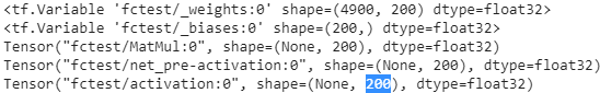
the dense layer’s output was a tensor of shape [batch size, 200]

tensorflow v1

# Implementing a CNN in TensorFlow low-level API by using tensorflow.compat.v1
import tensorflow.compat.v1 as tf
import numpy as np
 
def fc_layer(input_tensor,       # Tensor("Placeholder:0", shape=(None, 7, 7, 100), dtype=float32)
             name,               # name='fctest'
             n_output_units,     # n_output_units=200
             activation_fn=None):# activation_fn=tf.nn.relu
 
    with tf.variable_scope(name):
        input_shape = input_tensor.get_shape().as_list()[1:] # return [7, 7, 100]
        n_input_units = np.prod(input_shape) # return 4900 = 7*7*100
 
        # similar to model.add( keras.layers.Flatten() ) # since a dense network expects a 1D array of features for each instance
        if len(input_shape) > 1:
            input_tensor = tf.reshape(input_tensor, 
                                      shape=(-1, n_input_units)
                                     )#Tensor("fctest/Reshape:0", shape=(None,4900), dtype=float32)
  
        weights_shape = [n_input_units, n_output_units] #[4900, 200]
        # tf.compat.v1.get_variable
        #    # Gets an existing variable with these parameters or create a new one.
        weights = tf.get_variable(name='_weights',
                                  shape=weights_shape)
        print(weights)        # <tf.Variable 'fctest/_weights:0' shape=(4900, 200) dtype=float32>
        
        biases = tf.get_variable(name='_biases',
                                 initializer=tf.zeros(
                                                         shape=[n_output_units]
                                                     )
                                )
        print(biases)         # <tf.Variable 'fctest/_biases:0' shape=(200,) dtype=float32>
        
        # mat_shape(batches, 4900) x mat_shape(4900, 200) ==> mat_shape(batches, 200)
        layer = tf.matmul(input_tensor, weights)#shape(None, 200)
        print(layer)   # Tensor("fctest/MatMul:0", shape=(None, 200), dtype=float32)
        layer = tf.nn.bias_add(layer, biases,
                              name='net_pre-activation')
        print(layer)   # Tensor("fctest/net_pre-activation:0", shape=(None, 200), dtype=float32)
        
        if activation_fn is None:
            return layer
        
        layer = activation_fn(layer, name='activation')
        print(layer)    # Tensor("fctest/activation:0", shape=(None, 200), dtype=float32)
        return layer
 
    
## testing:
g = tf.Graph()
with g.as_default():
    x = tf.placeholder(tf.float32, shape=[None, 7, 7, 100]) #100 feature maps, each of size 7 × 7 (this is the feature map size
    
    fc_layer(x, name='fctest', n_output_units=200, 
             activation_fn=tf.nn.relu)
    
del g, x

for each instance 

 

tensorflow v2

import tensorflow as tf # tf.__version__ : '2.1.0'
from tensorflow import keras
import numpy as np

def fc_layer(input_tensor,       # Tensor("Placeholder:0", shape=(None, 7, 7, 100), dtype=float32)
             name,               # name='fctest'
             n_output_units,     # n_output_units=200
             activation_fn=None):# activation_fn=tf.nn.relu
    
    # print(input_tensor.get_shape().as_list()) # [None, 7, 7, 100]
    input_shape = input_tensor.get_shape().as_list()[1:] # # print(input_shape) # [7, 7, 100]
    n_input_units = np.prod(input_shape) # return 4900 = 7*7*100
    
    # similar to model.add( keras.layers.Flatten() ) # since a dense network expects a 1D array of features for each instance
    if len(input_shape) > 1:
        input_tensor = tf.reshape(input_tensor, 
                                  shape=(-1, n_input_units)
                                 )
        # print(input_tensor) # Tensor("lambda_7/Reshape:0", shape=(None, 4900), dtype=float32)
    
    initializer = tf.keras.initializers.RandomNormal(mean=0., stddev=1.)#########
    # tf.Variable :
    #   # The Variable() constructor requires an initial value for the variable, 
    #   # which can be a Tensor of any type and shape. This initial value defines the
    #   # type and shape of the variable. After construction, the type and shape of the
    #   # variable are fixed. The value can be changed using one of the assign methods
    weights = tf.Variable( initializer( shape=(n_input_units, n_output_units ) ), 
                           name='_weights')#########
    print(weights) # <tf.Variable '_weights:0' shape=(4900, 200) dtype=float32, numpy=
    
    
    biases = tf.Variable( initial_value=tf.zeros( shape=n_output_units ),
                          name='_bias')#########
    print(biases) # <tf.Variable '_bias:0' shape=(200,) dtype=float32, numpy=

    
    layer = tf.matmul(input_tensor, weights)
    print(layer) # Tensor("lambda_6/MatMul:0", shape=(None,  200), dtype=float32)
    
    # layer=layer+biases # applying broadcasting
    # OR
    layer = tf.nn.bias_add( layer, biases,
                            name='net_pre-activation')
    print(layer) # Tensor("net_pre-activation_11:0", shape=(None, 200), dtype=float32)
    
    
    if activation_fn is None:
        return layer
    
    layer = activation_fn(layer, name='activation') # similar to # tf.keras.activations.get( 'activation' )
    print(layer) # Tensor("lambda_6/activation:0", shape=(None, 200), dtype=float32)
    return layer 
    
x_in = keras.layers.Input(shape=(7,7,100), batch_size=None, name='input')
fc_layer(x_in, name='fctest', n_output_units=200, activation_fn=tf.nn.relu)

     To understand this, let’s look at an example: suppose a dense layer with 200 neurons(n_neurons=200 or C_out=200) sits on top of a convolutional layer that outputs 100 feature maps or channels(is the C_in of this dense layer), each of size 7 × 7 (this is the feature map size(input_tensor), not the kernel size). Each neuron will compute a weighted sum of all 100 × 7×7 activations from the convolutional layer (plus a bias term, 1 bias per neurons or per output chanel or per feature map in C_out ).
###
    for this dense layer, 100 channels * input_X.shape(7,7) https://blog.csdn.net/Linli522362242/article/details/108414534
tf.matmul( input_tensor.shape(batches, 4900), weights.shape=(4900, 200) )==>shape=( batches OR None, 200)  +b.shape(200, since 1 bias per neurons or output chanels C_out ) ==>(None, 200)==> 200 numbers
### VS a Convolution layer
#########################################################

Numpy examples. To make the discussion above more concrete, lets express the same ideas but in code and with a specific example. Suppose that the input volume is a numpy array X. Then:

• A depth column (or a fibre) at position (axis_0,axis_1) would be the activations X[axis_0,axis_1,:].
• A depth slice, or equivalently an activation map at depth d would be the activations X[:,:,d].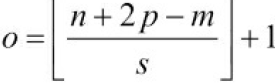
  

Conv Layer Example. Suppose that the input volume X has shape X.shape: (11,11,4). Suppose further that we use no zero padding (P=0), that the filter size is F=5x5, and that the stride is S=2. The output volume would therefore have spatial size (11+2*0-5)/2+1 = 4, giving a volume with width and height of 4. The activation map in the output volume (call it V), would then look as follows (only some of the elements are computed in this example): W.shape(5,5,C_in=4, C_out)

• V[0,0,0] = np.sum(X[:5,:5,:] * W0) + b0  (example of going along axis_0 ) and the ' * ' does element-wise multiplication
• V[1,0,0] = np.sum(X[2:7,:5,:] *W0) + b0
• V[2,0,0] = np.sum(X[4:9,:5,:] *W0) + b0
• V[3,0,0] = np.sum(X[6:11,:5,:]*W0) + b0
  1 bias per neuron or per output chanel in C_out
  note np.sum(X[:5,:5,_:_] * W0) ==> sum(X[:5,:5,0]*W0)+sum(X[:5,:5,1]*W0)+sum(X[:5,:5,2]*W0)+sum(X[:5,:5,4-1]*W0) #along deep #C_in=4

     Remember that in numpy, the operation * above denotes elementwise multiplication between the arrays. Notice also that the weight vector W0 is the weight vector of that neuron and b0 is the bias. Here, W0 is assumed to be of shape W0.shape: (5,5,4), since the filter size is 5 and the depth of the input volume is 4. Notice that at each point, we are computing the dot product as seen before in ordinary neural networks. Also, we see that we are using the same weight and bias (due to parameter sharing), and where the dimensions along the width are increasing in steps of 2 (i.e. the stride).
To construct a second activation map in the output volume, we would have:

• V[0,0,1] = np.sum(X[:5,:5,:] * W1) + b1 (example of going along axis_0 ) and the ' * ' does element-wise multiplication   
• V[1,0,1] = np.sum(X[2:7,:5,:] * W1) + b1
• V[2,0,1] = np.sum(X[4:9,:5,:] * W1) + b1
• V[3,0,1] = np.sum(X[6:11,:5,:]* W1) + b1  
•  
• V[0,1,1] = np.sum(X[:5,2:7,:]  * W1) + b1 ( example of going along axis_1 in the second activation map) 
• V[2,3,1] = np.sum(X[4:9,6:11,:] * W1) + b1 ( or along both(axis_0, axis_1) )

     where we see that we are indexing into the second depth dimension in V (at index 1) because we are computing the second activation map, and that a different set of parameters (W1) is now used. In the example above, we are for brevity leaving out some of the other operations the Conv Layer would perform to fill the other parts of the output array V. Additionally, recall that these activation maps are often followed elementwise through an activation function such as ReLU, but this is not shown here.

#########################################################

convert the CNN (the last layer is a dense layer) into an convolutional layer or FCN(Fully Convolutional Networks)

     To understand this, let’s look at an example: suppose a dense layer with 200 neurons(n_neurons=200 or C_out=200) sits on top of a convolutional layer that outputs 100 feature maps or channels
(###
       input_tensor, : Tensor("Placeholder:0", shape=(None, 7, 7, 100), dtype=float32)
###)
,each of size 7 × 7 (this is the feature map size(input_tensor), not the kernel size). Each neuron will compute a weighted sum
(###
     layer=tf.matmul(input_tensor.shape=(None, 4900), weights.shape=(4900, 200))
###)
of all 100 × 7×7 activations from the convolutional layer (plus a bias term, 1 bias per neurons or per output chanel or per feature map in C_out )
(###
      layer = tf.nn.bias_add( layer, biases.shape=(200,), name='net_pre-activation' )
      output.shape : (None_batch size, 200)
###)
. Now let’s see what happens if we replace the dense layer with a convolutional layer using 200 filters(since), each of size 7 × 7, and with "valid" padding(p=0). This layer will output 200 feature maps(since), each 1 × 1 (since the kernel is exactly the size of the input feature maps
###
      conv_layer(x.shape=(None, 7, 7, 100), name='convtest', kernel_size=(7, 7), n_output_channels=200) and strides=(1,1)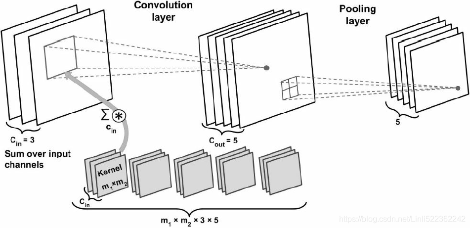
and
include  ( the number of output feature maps >=1) :
the current output feature map index: k in  and compute the sum of the element-wise product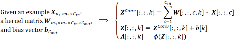

cp15_Classifying Images with Deep Convolutional NN_Loss_Cross Entropy_ax.text_mnist_ CelebA_Colab_ck
https://blog.csdn.net/Linli522362242/article/details/108414534
In each channel, the Input * Kernel is using element-wise multiplication, then sum all elements in the result of multiplication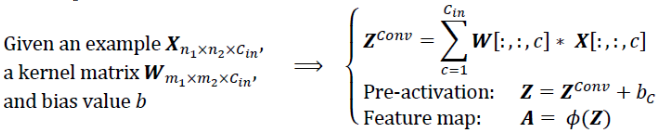
 1 output Channels OR C_out=1
and ==>output shape (for each output feature map k)=(7-2*0-7)/1+1=1
###
and we are using "valid" padding). In other words, it will output 200 numbers ([batch size, 1, 1, 200]), just like the dense layer did([batch size, 200]); and if you look closely at the computations performed by a convolutional layer, you will notice that these numbers will be precisely the same as those the dense layer produced. The only difference is that the dense layer’s output was a tensor of shape [batch size, 200], while the convolutional layer will output a tensor of shape [batch size, 1, 1, 200].

      To convert a dense layer to a convolutional layer, the number of filters in the convolutional layer must be equal to the number of units in the dense layer, the filter size must be equal to the size of the input feature maps, and you must use "valid" padding. The stride may be set to 1 or more, as we will see shortly.

     Why is this important? Well, while a dense layer expects a specific input size (since it has one weight per input feature, e.g. 49), a convolutional layer will happily process images of any size(e.g. 7x7)（###There is one small exception: a convolutional layer using "valid" padding will complain if the input size is smaller than the kernel size.###） (however, it does expect its inputs to have a specific number of channels, since each kernel contains a different set of weights for each input channel). Since an FCN(Fully Convolutional Networks) contains only convolutional layers (and pooling layers, which have the same property), it can be trained and executed on images of any size!

     For example, suppose we’d already trained a CNN((Convolutional Neural Networks)) for flower classification and localization. It was trained on 224 × 224 images, and it outputs 10 numbers:

• outputs 0 to 4 are sent through the softmax activation function, and this gives the class probabilities (one per class);
• output 5 is sent through the logistic activation function, and this gives the objectness score;
• outputs 6 to 9 do not use any activation function, and they represent the bounding box’s center coordinates, as well as its height and width.

We can now convert its dense layers to convolutional layers. In fact, we don’t even need to retrain it; we can just copy the weights from the dense layers to the convolutional layers! Alternatively, we could have converted the CNN(Convolutional neural networks) into an FCN(Fully Convolutional Networks, e.g. dense) before training.

Figure 14-25. The same fully convolutional network processing a small image (left) and a large one (right)

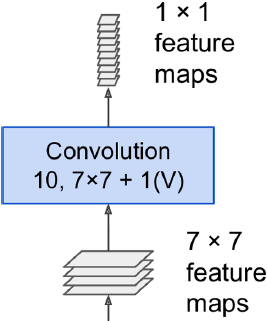
     Now suppose the last convolutional layer before the output layer (also called the bottleneck layer) outputs 7×7x4 feature maps when the network is fed a 224 × 224 image (see the left side of Figure 14-25). Since the dense output layer was replaced by a convolutional layer using 10 filters of size 7 × 7
###
https://blog.csdn.net/Linli522362242/article/details/108396485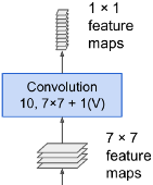
==> weight.shape=(7, 7, 4, 10 since n_output_channels=10)
###,
with "valid" padding(p=0) and stride 1, the output will be composed of 10 features maps, each of size 1 × 1 (since (7 + 2*0 - 7)/1 + 1 = 1)

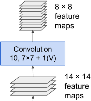
     If we feed the FCN a 448 × 448 image (see the right side of Figure 14-25), the bottleneck layer will now output 14×14x4 feature maps.
(###This assumes we used only "same" padding in the network: indeed, "valid" padding would reduce the size of the feature maps. Moreover, 448 can be neatly divided by 2 several times until we reach 7 (448/ (2^6)=448/64=7), without any rounding error. If any layer uses a different stride than 1 or 2, then there may be some rounding error, so again the feature maps may end up being smaller.###)
Since the dense output layer was replaced by a convolutional layer using 10 filters of size 7 × 7
###
==> weight.shape=(7, 7, 4, 10 since n_output_channels=10) 

###, with "valid" padding(p=0) and stride 1, the output will be composed of 10 features maps, each of size 8 × 8 (since (14 + 2*0 - 7)/1 + 1 = 8). In other words, the FCN will process the whole image only once, and it will output an 8 × 8 grid where each cell contains 10 numbers (

• 5 class probabilities,
• 1 objectness score, and
• 4 bounding box coordinates).

It’s exactly like taking the original CNN and sliding it across the image using 8 steps per row and 8 steps per column. To visualize this, imagine chopping the original image into a 14 × 14 grid, then sliding a 7 × 7 window across this grid, stride s=1; there will be 8 × 8 = 64 possible locations for the window, hence 8 × 8 predictions. However, the FCN approach is much more efficient, since the network only looks at the image once. In fact, You Only Look Once (YOLO) is the name of a very popular object detection architecture, which we’ll look at next.

#####################################################

the dense layer’s output was a tensor of shape [batch size, 10]

# Implementing a CNN in TensorFlow low-level API by using tensorflow.compat.v1
import tensorflow.compat.v1 as tf
import numpy as np
 
def fc_layer(input_tensor,       # Tensor("Placeholder:0", shape=(None, 7, 7, 4), dtype=float32)
             name,               # name='fctest'
             n_output_units,     # n_output_units=10
             activation_fn=None):# activation_fn=tf.nn.relu
 
    with tf.variable_scope(name):
        input_shape = input_tensor.get_shape().as_list()[1:] # return [7, 7, 4]
        n_input_units = np.prod(input_shape) # return 196 = 7*7*4
 
        if len(input_shape) > 1:
            input_tensor = tf.reshape(input_tensor, 
                                      shape=(-1, n_input_units)
                                     )#Tensor("fctest/Reshape:0", shape=(None,196), dtype=float32)
  
        weights_shape = [n_input_units, n_output_units] #[196, 10]
        weights = tf.get_variable(name='_weights',
                                  shape=weights_shape)
        print(weights)        # <tf.Variable 'fctest/_weights:0' shape=(196, 10) dtype=float32>
        
        biases = tf.get_variable(name='_biases',
                                 initializer=tf.zeros(
                                                         shape=[n_output_units]
                                                     )
                                )
        print(biases)         # <tf.Variable 'fctest/_biases:0' shape=(10,) dtype=float32>
        
        # mat_shape(batches, 196) x mat_shape(196, 10) ==> mat_shape(batches, 10)
        layer = tf.matmul(input_tensor, weights)#shape(None, 10)
        print(layer)   # Tensor("fctest/MatMul:0", shape=(None, 10), dtype=float32)
        layer = tf.nn.bias_add(layer, biases,
                              name='net_pre-activation')
        print(layer)   # Tensor("fctest/net_pre-activation:0", shape=(None, 10), dtype=float32)
        
        if activation_fn is None:
            return layer
        
        layer = activation_fn(layer, name='activation')
        print(layer)    # Tensor("fctest/activation:0", shape=(None, 10), dtype=float32)
        return layer
 
    
## testing:
g = tf.Graph()
with g.as_default():
    x = tf.placeholder(tf.float32, shape=[None, 7, 7, 4])
    
    fc_layer(x, name='fctest', n_output_units=10, 
             activation_fn=tf.nn.relu)
    
del g, x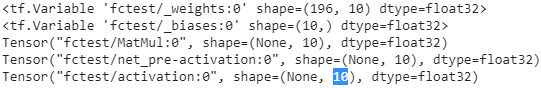

## testing:
g = tf.Graph()
with g.as_default():
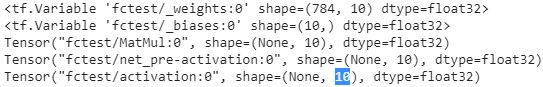
    x = tf.placeholder(tf.float32, shape=[None, 14, 14, 4])
    
    fc_layer(x, name='fctest', n_output_units=10, 
             activation_fn=tf.nn.relu)
    
del g, x

14*14*4channels=784 

 

the convolutional layer will output a tensor of shape [batch size, 1, 1, 10]

# Implementing a CNN in TensorFlow low-level API by using tensorflow.compat.v1
import tensorflow.compat.v1 as tf
import numpy as np
 
 
## wrapper functions 
                             
def conv_layer(input_tensor, # Tensor("Placeholder:0", shape=(None, 7, 7, 4), dtype=float32)
               name,              # name='convtest'
               kernel_size,       # kernel_size=(7, 7)
               n_output_channels, # n_output_channels=10
               padding_mode='VALID', strides=(1, 1, 1, 1)):
    with tf.variable_scope(name):# convtest/
        
        ## get n_input_channels:
        ##   input tensor shape: 
        ##   [batch x width x height x channels_in]
        input_shape = input_tensor.get_shape().as_list() #return [None, 7, 7, 4]
        n_input_channels = input_shape[-1]
 
                        # [ width, height,                C_in, C_out ]
        weights_shape = (list(kernel_size) + [n_input_channels, n_output_channels])
        weights = tf.get_variable(name='_weights', shape=weights_shape)
        print(weights)     #<tf.Variable 'convtest/_weights:0' shape=(7, 7, 4, 10) dtype=float32>
        
        ################################################    
        conv = tf.nn.conv2d(input=input_tensor, 
                            filter=weights,
                            strides=strides, 
                            padding=padding_mode)      #padding_mode='VALID' ==>p=0 
        print(conv)       #Tensor("convtest/Conv2D:0", shape=(None, 1, 1, 10), dtype=float32)
                          # output shape 1 = (7 + 2*0 - 7)/1 +1=1 
        ################################################ 
        biases = tf.get_variable(name='_biases',
                                 initializer=tf.zeros(
                                                         shape=[n_output_channels]
                                                     )
                                )
        print(biases)      #<tf.Variable 'convtest/_biases:0' shape=(10,) dtype=float32>
        
        conv = tf.nn.bias_add(conv, biases, 
                              name='net_pre-activation')
        print(conv)#Tensor("convtest/net_pre-activation:0", shape=(None,1,1,10), dtype=float32)
        
        #################################################
        conv = tf.nn.relu(conv, name='activation')
        print(conv)# Tensor("convtest/activation:0", shape=(None, 1, 1, 10), dtype=float32)
        
        return conv
    
 
## testing
g = tf.Graph()
with g.as_default():
    x = tf.placeholder(tf.float32, shape=[None, 7, 7, 4])
    conv_layer(x, name='convtest', kernel_size=(7, 7), n_output_channels=10)
    
del g, x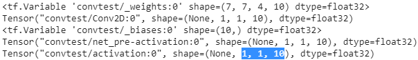

 <==

the convolutional layer will output a tensor of shape [batch size, 8, 8, 10]

## testing
g = tf.Graph()
with g.as_default():
    x = tf.placeholder(tf.float32, shape=[None, 14, 14, 4])
    conv_layer(x, name='convtest', kernel_size=(7, 7), n_output_channels=10)
    
del g, x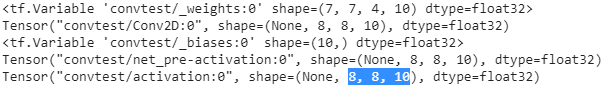

 <==

#####################################################

You Only Look Once (YOLO)

     YOLO is an extremely fast and accurate object detection architecture proposed by Joseph Redmon et al. in a 2015 paper,(Joseph Redmon et al., “You Only Look Once: Unified, Real-Time Object Detection,https://arxiv.org/pdf/1506.02640.pdf” Proceedings of the IEEE Conference on Computer Vision and Pattern Recognition (2016): 779–788.) and subsequently improved in 2016(YOLOv2, Joseph Redmon and Ali Farhadi, “YOLO9000: Better, Faster, Stronger, https://arxiv.org/pdf/1612.08242.pdf” Proceedings of the IEEE Conference on Computer Vision and Pattern Recognition (2017): 6517–6525.) and in 2018(Joseph Redmon and Ali Farhadi, “YOLOv3: An Incremental Improvement, https://pjreddie.com/media/files/papers/YOLOv3.pdf” arXiv preprint arXiv:1804.02767 (2018).). It is so fast that it can run in real time on a video, as seen in Redmon’s demo.

####################################################################################

How to implement a YOLO (v3) object detector from scratch in PyTorch: Part 1
https://blog.paperspace.com/how-to-implement-a-yolo-object-detector-in-pytorch/

     The official title of YOLO v2 paper seemed if YOLO was a milk-based health drink for kids rather than a object detection algorithm. It was named “YOLO9000: Better, Faster, Stronger”. For it’s time YOLO 9000 was the fastest, and also one of the most accurate algorithm. However, a couple of years down the line and it’s no longer the most accurate with algorithms like RetinaNet, and SSD outperforming it in terms of accuracy. It still, however, was one of the fastest.

What is YOLO?

     YOLO stands for You Only Look Once. It's an object detector that uses features learned by a deep convolutional neural network to detect an object. Before we get out hands dirty with code, we must understand how YOLO works.

     The network downsamples the image by a factor called the stride of the network. For example, if the stride of the network is 32, then an input image of size 416 x 416 will yield an output of size 13 x 13 (416/32=13). Generally, stride of any layer in the network is equal to the factor倍数 by which the output of the layer is smaller than the input image to the network.

Interpreting the output

     Typically, (as is the case for all object detectors) the features learned by the convolutional layers are passed onto a classifier/regressor which makes the detection prediction (coordinates of the bounding boxes, the class label.. etc).

In YOLO, the prediction is done by using a convolutional layer which uses 1 x 1 convolutions.

     1x1 convolution. As an aside, several papers use 1x1 convolutions, as first investigated by Network in Network. Some people are at first confused to see 1x1 convolutions especially when they come from signal processing background. Normally signals are 2-dimensional so 1x1 convolutions do not make sense (it’s just pointwise scaling). However, in ConvNets this is not the case because one must remember that we operate over 3-dimensional volumes, and that the filters always extend through the full depth of the input volume. For example, if the input is [32x32x3] then doing 1x1 convolutions would effectively be doing 3-dimensional dot products (since the input depth is 3 channels).https://cs231n.github.io/convolutional-networks/#conv

     Now, the first thing to notice is our output is a feature map. Since we have used 1 x 1 convolutions, the size of the prediction map is exactly the size of the feature map before it( OR The feature map produced by this kernel has identical height and width of the previous feature map). In YOLO v3 (and it's descendants), the way you interpret this prediction map is that each cell can predict a fixed number of bounding boxes.

     Though the technically correct term to describe a unit in the feature map would be a neuron, calling it a cell makes it more intuitive in our context.

YOLO v3 network Architecture

https://towardsdatascience.com/yolo-v3-object-detection-53fb7d3bfe6b

https://blog.paperspace.com/how-to-implement-a-yolo-object-detector-in-pytorch/

Detection at three Scales

     The newer architecture boasts of residual skip connections, and upsampling. The most salient feature of v3 is that it makes detections at three different scales. YOLO is a fully convolutional network and its eventual output is generated by applying a 1 x 1 kernel on a feature map. In YOLO v3, the detection is done by applying 1 x 1 detection kernels on feature maps of three different sizes at three different places in the network.

https://blog.csdn.net/Linli522362242/article/details/108396485

 Figure 14-17. ResNet architecture

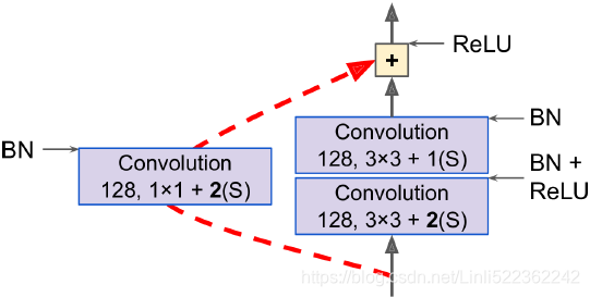Figure 14-18. Skip connection when changing feature map size and depth

Darknet-53

在基本的图像特征提取方面，YOLO3采用了称之为Darknet-53的网络结构（含有53个卷积层），它借鉴了残差网络residual network的做法，在一些层之间设置了快捷链路（shortcut connections）

 Darknet-53网络采用256*256*3作为输入，最左侧那一列的1、2、8等数字表示多少个重复的残差组件。每个残差组件有两个卷积层和一个快捷链路，示意图如下：

    The newer architecture boasts of residual skip connections, and upsampling. The most salient [ˈseɪliənt]显著的 feature of v3 is that it makes detections at three different scales. YOLO is a fully convolutional network and its eventual output is generated by applying a 1 x 1 kernel on a feature map. In YOLO v3, the detection is done by applying 1 x 1 detection kernels on feature maps of three different sizes at three different places in the network.

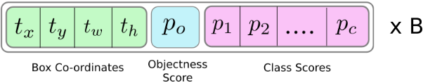
     The shape of the detection kernel is 1 x 1 x ( B x (5 + C) ). Here B is the number of bounding boxes a cell on the feature map can predict,

• “5” is for the 4 bounding box attributes(describe the center coordinates, the dimensions) and one object confidence(also called the objectness score) and
• C is the number of classes.
• In YOLO v3 trained on COCO, B = 3 (means YOLO v3 predicts 3 bounding boxes for every cell)and C = 80, so the kernel size is 1 x 1 x 255. ###255=3*(5+80)### The feature map produced by this kernel has identical height and width of the previous feature map, and has detection attributes along the depth as described above.

     You expect each cell of the feature map to predict an object through one of it's bounding boxes(1-to-n) if the center of the object falls in the receptive field of that cell
--我的理解：假如某个对象的中心落在一个local Receptive field（coresponding to an specified cell in the feature map）中，而这个local Receptive field存在多个bounding box, 那么我们就能通过feature map的这个specified cell对应的local receptive fileld中的一个bounding box去预测对象
--If the center of an object falls in a local Receptive field (corresponding to an specified cell in the feature map), and there are multiple bounding boxes in the local Receptive field, then we can predict the object through one of the local receptive fileld's bounding boxes and the local receptive fileld related to the specified cell in the feature map. 
(local Receptive field is the region of the input image visible to the cell in the feature map. Refer to the link on convolutional neural networks for further clarification).
#########################
cp15_Classifying Images with Deep Convolutional NN_Loss_Cross Entropy_ax.text_mnist_ CelebA_Colab_ck
https://blog.csdn.net/Linli522362242/article/details/108414534

     As you can see in the following image, a CNN computes feature maps from an input image, where each element comes from a local patch of pixels in the input image: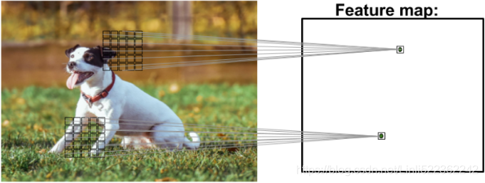

     This local patch of pixels is referred to as the local receptive field（~~coresponding to one cell in the feature map）. 
( the picture can be treated as an whole receptive field~~corresponding to~~an feature map）

#########################

     This has to do with how YOLO is trained, where only one bounding box is responsible for detecting any given object. First, we must ascertain[ˌæsərˈteɪn]确定 which of the cells(in the feature map) this bounding box belongs to.

     To do that, we divide the input image into a grid of dimensions equal to that of the final feature map.

     Let us consider an example below, where the input image is 416 x 416, and stride of the network is 32. As pointed earlier, the dimensions of the feature map will be 13 x 13 (13=416/32). We then divide the input image into 13 x 13 cells (each cell will be  32x32,  whole input image ~~ corresponding to a feature map). 
  

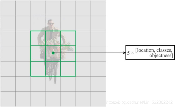
      Then, the cell (on the input image) containing the center of the ground truth box of an object is chosen to be the one responsible for predicting the object. In the image, it is the cell which marked red, which contains the center of the ground truth box (marked yellow). # dog figure

     Now, the red cell is the 7th cell in the 7th row on the grid. We now assign the 7th cell in the 7th row on the feature map (corresponding cell on the feature map) as the one responsible for detecting the dog.

     Note that the cell we're talking about here is a cell on the prediction feature map. We divide the input image into a grid just to determine which cell of the prediction feature map is responsible for prediction（Separately, we use the term "cell" in the (prediction) feature map, use term "local receptive field" in the input image, whole feature map is corresponding to one input image）

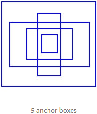
Anchor Boxes

     It might make sense to predict the width and the height of the bounding box, but in practice, that leads to unstable gradients during training. Instead, most of the modern object detectors predict log-space transforms, or simply offsets to pre-defined default bounding boxes called anchors.

     Then, these transforms are applied to the anchor boxes(pre-defined default bounding boxes) to obtain the prediction. YOLO v3 has three anchors, which result in prediction of three bounding boxes per cell( this cell is in current prediction feature map ).

     Coming back to our earlier question, the bounding box responsible for detecting the dog will be the one whose anchor has the highest IoU with the ground truth box.

Making Predictions Formula

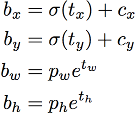
The following formulae describe how the network output is transformed to obtain bounding box predictions.
     The network predicts 4 coordinates for each bounding box, tx, ty, tw, th. If the cell is offset from the top left corner of the image by (cx, cy) and the bounding box prior has width and height pw, ph, then the predictions correspond to:

The blue box below is the predicted bounding box(the (predicted) ground-truth box) and the dotted rectangle is the anchor box(bounding box priors).

                                                                      these transforms are applied to the anchor boxes(pre-defined default bounding boxes) to obtain the prediction
<== <==In YOLO v3 trained on COCO, B = 3 (means YOLO v3 predicts 3 bounding boxes for every cell)

• bx, by, bw, bh are the x,y center co-ordinates, width and height of our prediction(are the predicted bounding box). 
   
• tx, ty, tw, th is what the network outputs(are predictions made by YOLO). 
   
• cx, cy is the top-left corner of the grid cell of the anchor(bounding box priors).
• pw and ph are anchor's dimensions for the box.
• cx, cy, pw, ph are normalized by the image width and height
• 

     Figure 2(above left). Bounding boxes with dimension priors and location prediction. We predict the width and height of the box as offsets from cluster centroids. We predict the center coordinates of the box relative to the location of filter application using a sigmoid function

YOLOv3 applies the logistic sigmoid activation function to the bounding box coordinatesto ensure they remain in the 0 to 1 range.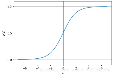https://blog.csdn.net/Linli522362242/article/details/96480059. 

Objectness Score

     Object score represents the probability that an object is contained inside a bounding box. It should be nearly 1 for the red and the neighboring grids, whereas almost 0 for, say, the grid at the corners.

The objectness score is also passed through a sigmoid, as it is to be interpreted as a probability.

     During training we use sum of squared error loss. If the ground truth (for some coordinate prediction) is  (is one of x, y, h, w), but the (the ground truth box coresponding to the specified ground truth) anchor box's bx, by, bw, bh are in our training set, so we need to convert them to the ground truth  since from Yolo we get the ). our gradient is the ground truth value (computed from the ground truth box) minus our prediction: . This ground truth value can be easily computed by inverting the equations above
( tw=log(bw/pw), th=log(bh/ph),
). ==>  minimize the loss ==>optimal model parameters(e.g. weights)

     YOLOv3 predicts an objectness score for each bounding box using logistic regression. This should be 1 if the bounding box prior overlaps a ground truth object by more than any other bounding box prior(### Suppose current ground truth object has a real anchor, and the IOU between the predicted anchor (the bounding box prior) we currently use and the real anchor and the real anchor is larger than other predicted anchors, then the objectness score should be set to 1, that is, the predicted anchor we currently use is the best for predicting the current ground truth object ###). 

     If the bounding box prior is not the best but does overlap a ground truth object by more than some threshold we ignore the prediction, following. We use the threshold of 0.5. Unlike our system only assigns one bounding box prior for each ground truth object. If a bounding box prior is not assigned to a ground truth object it incurs no loss for coordinate or class predictions, only objectness.（###When predicting, we use multiple anchors, and then use objectness score to find the most suitable anchor for predicting the object. (even if other anchors' IOU> threshold=0.5 we still have to discard them. Furthermore, even if those anchors are not assigned to any ground truth object, they do not cause any loss to the object category prediction)###）

Center Coordinates

     Notice we are running our center coordinates prediction through a sigmoid function. This forces the value of the output to be between 0 and 1. Why should this be the case? Bear with me.

Normally, YOLO doesn't predict the absolute coordinates of the bounding box's center. It predicts offsets which are:

• Relative to the top left corner of the grid cell which is predicting the object.   ### tx, ty

• Normalised by the dimensions of the cell from the feature map, which is, 1. ### cx, cy, pw, ph are normalized by the image width and height

          Let us consider an example below, where the input image is 416 x 416, and stride of the network is 32. As pointed earlier, the dimensions of the feature map will be 13 x 13 (13=416/32). We then divide the input image into 13 x 13 cells (each cell will be  32x32,  whole input image ~~ corresponding to a feature map). 

sigmoid function

     For example, consider the case of our dog image. If the prediction for center is (tx, ty)= (0.4, 0.7), then this means that the center lies at (b_x = tx+cx, b_y=ty+cy)=(6.4, 6.7) on the 13 x 13 feature map. (Since the top-left co-ordinates of the red cell are (cx, cy)=(6,6)).

     But wait, what happens if the predicted x,y co-ordinates are greater than one, say (tx, ty)=(1.2, 0.7). This means center lies at (b_x = tx+cx, b_y=ty+cy)= (7.2, 6.7) . Notice the center now lies in cell just right to our red cell, or the 8th cell in the 7th row( 7th =[6.0, 7.0], 8th=[7.0, 8.0] ). This breaks theory behind YOLO because if we postulate假定 that the red box is responsible for predicting the dog, the center of the dog must lie in the red cell, and not in the one beside it.

     Therefore, to remedy this problem, the output is passed through a sigmoid function, which squashes the output in a range from 0 to 1, effectively keeping the center in the grid which is predicting.

Dimensions of the Bounding Box
           pw and ph are anchor's dimensions for the bounding box.

     The dimensions of the bounding box are predicted by applying a log-space transform(, ) to the output(tw,th) and then multiplying with an anchor.
==><==The blue box is the predicted bounding box and the dotted rectangle is the anchor box( bounding box priors).
How the detector output is transformed to give the final prediction. Image Credits. http://christopher5106.github.io/

     The network downsamples the image by a factor called the stride of the network. For example, if the stride of the network is 32, then an input image of size 416 x 416 will yield an output of size 13 x 13 (416/32=13). Generally, stride of any layer in the network is equal to the factor倍数 by which the output of the layer is smaller than the input image to the network.

cx, cy is the top-left corner of the grid cell of the anchor(bounding box priors).
pw and ph are anchor's dimensions for the bounding box. cx, cy, pw, ph are normalized by the image width and height.

     The predictions, bx, by, bw, bh, are normalised by the height and width of the image. (Training labels are chosen this way). So, if the model output tell us the values (tw, th) and the selected anchor ( its dimensions are pw and ph) then we get the predictions  ==> the predicted bounding box containing the dog are (bw, bh)=(0.3, 0.8) ==> the actual width and height on 13 x 13 feature map is (13 x 0.3, 13 x 0.8).

why (13 x 0.3, 13 x 0.8)? 

     The original image is downsampled in the Yolo model (which can be understood as scaling or Shrink the image) to obtain the feature maps of different sizes (13x13, 26x26, 52x52). If the obtained feature map is 13x13, that is to say, the original image is reduced to 13x13, thus bw and by need to be divided by 13 on 13 x 13 feature map, tw = log(bw/13 / pw) and th=log(bh/13 /ph) ==> bw = pw * *13, bh = ph * *13 and the selected anchor' dimension (pw , ph) we the actual value.
( tw=log(bw/pw), th=log(bh/ph),
     Further more the bx and by are also divided by 13 on on 13 x 13 feature map, thus  also need to be multiplied by 13.

Class Confidences

     Class confidences represent the probabilities of the detected object belonging to a particular class (Dog, cat, banana, car etc). Before v3, YOLO used to softmax the class scores.

     However, that design choice has been dropped in v3, and authors have opted for using sigmoid(YOLO v3 used) instead. The reason is that Softmaxing class scores assume that the classes are mutually exclusive. In simple words, if an object belongs to one class, then it's guaranteed it cannot belong to another class. This is true for COCO database on which we will base our detector.

#######################################
04_TrainingModels_04_gradient decent with early stopping for softmax regression_ entropy_Gini : https://blog.csdn.net/Linli522362242/article/details/104124771
TIP
     The Softmax Regression classifier predicts only one class at a time (i.e., it is multiclass, not multioutput) so it should be used only with mutually exclusive classes such as different types of plants. You cannot use it to recognize multiple people in one picture.
#######################################

     However, this assumptions may not hold when we have classes like Women and Person. This is the reason that authors have steered clear of using a Softmax activation.

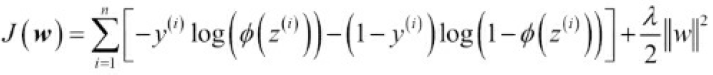
     Instead, independent logistic classifiers are used and binary cross-entropy loss is used. Because there may be overlapping labels for multilabel classification such as if the YOLOv3 is moved to other more complex domain such as Open Images Dataset.
https://blog.csdn.net/Linli522362242/article/details/108414534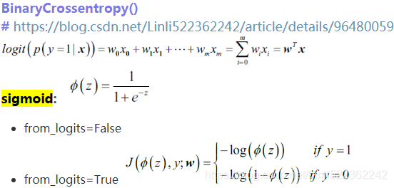

预测对象类别
https://blog.csdn.net/Linli522362242/article/details/96480059

Prediction across different scales.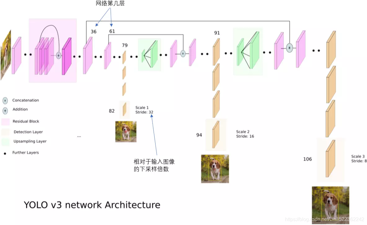

     YOLO v3 makes prediction across 3 different scales. The detection layer is used make detection at feature maps of three different sizes, having strides 32, 16, 8 respectively. This means, with an input of 416 x 416, we make detections on scales 13 x 13 (416/32=13), 26 x 26 (416/16=26) and 52 x 52(416/8=52).

     The network downsamples the input image until the first detection layer, where a detection is made using feature maps of a layer with stride 32. Further, layers are upsampled by a factor of 2 and concatenated with feature maps of a previous layers having identical feature map sizes. Another detection is now made at layer with stride 16. The same upsampling procedure is repeated, and a final detection is made at the layer of stride 8.

     The first detection is made by the 82nd layer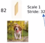. For the first 81 layers, the image is down sampled by the network, such that the 81st layer 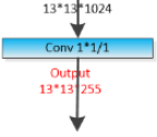has a stride of 32. If we have an image of 416 x 416, the resultant feature map would be of size 13x13 (416/32=13). One detection is made here using the 1 x 1 detection kernel (kernel size=1x1x( Bx(5+C) )=1x1x(3 bboxs x(5+80classes))=1x1x255 (### tf.reshape ###) and strides=1, padding = 'same' , giving us a detection feature map of 13 x 13 x 255.https://towardsdatascience.com/yolo-v3-object-detection-53fb7d3bfe6b

     Then, the feature map from layer 79 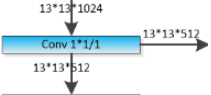is subjected to a few convolutional layers before 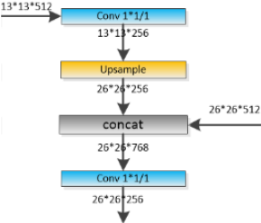being up sampled by 2x (### UpSampling2D(size=(2, 2)) ###) to dimensions of 26 x 26. This feature map is then depth concatenated(### Concatenate()([x, x_concat]) ###) with the feature map from layer 61. Then the combined feature maps is again subjected a few 1 x 1/strides=1 and 3x3/strides=1 convolutional layers to fuse the features from the earlier layer (61...<==26x26x52).==> 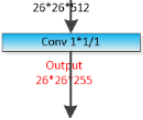==>Then, the second detection is made by the 94th layer, yielding a detection feature map of 26 x 26 x 255.

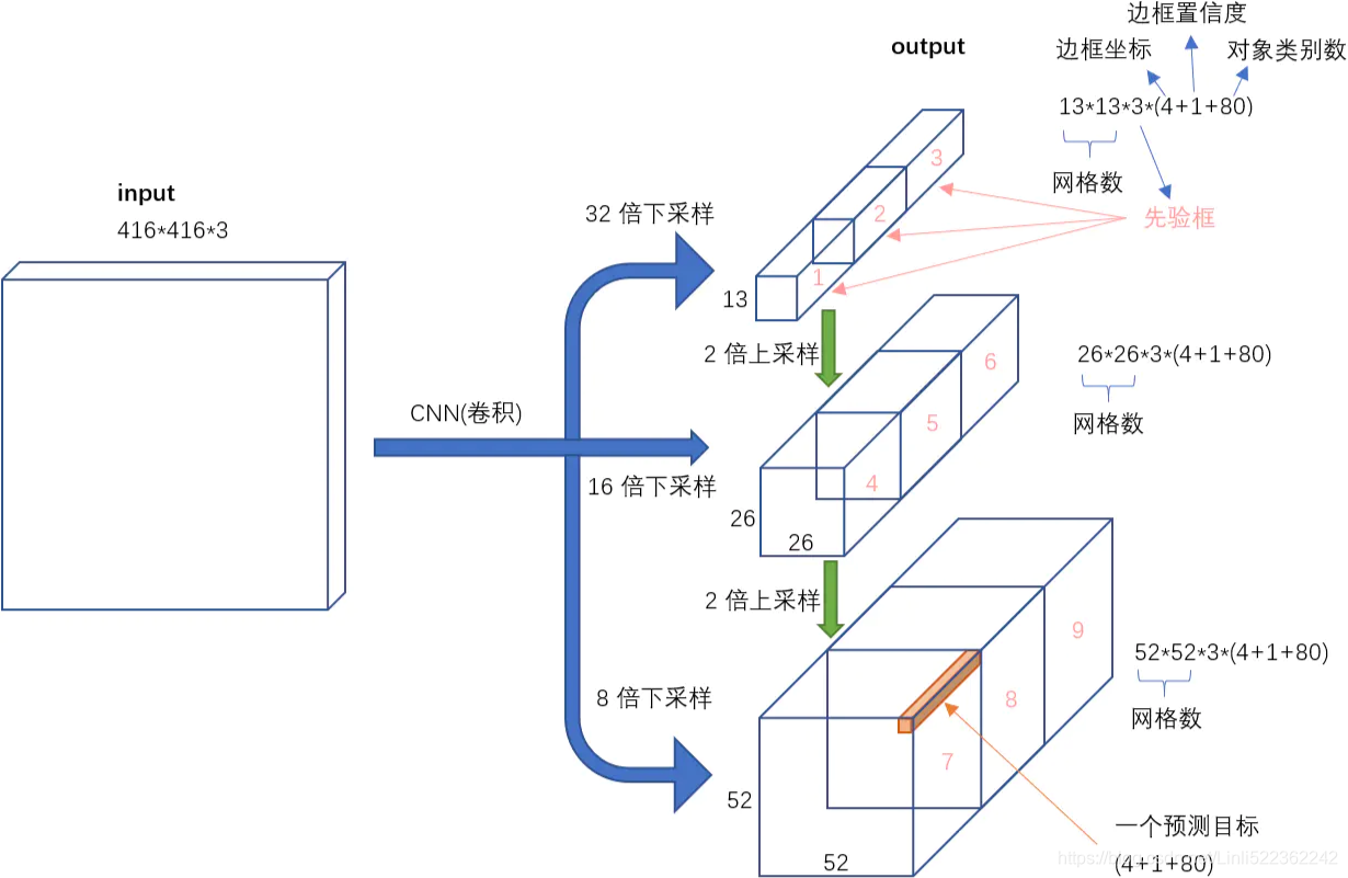
我们看一下YOLO3共进行了多少个预测。对于一个416*416的输入图像，在每个尺度的特征图的每个网格设置3个先验框，总共有 13*13*3 + 26*26*3 + 52*52*3 = 10647 个预测。每一个预测是一个(4+1+80)=85维向量，这个85维向量包含边框坐标（4个数值），边框置信度（1个数值），对象类别的概率（对于COCO数据集，有80种对象）。

对比一下，YOLO2采用13*13*5 = 845个预测，YOLO3的尝试预测边框数量增加了10多倍，而且是在不同分辨率上进行，所以mAP以及对小物体的检测效果有一定的提升。

Choice of anchor boxes and Better at detecting smaller objects

     The upsampled layers concatenated with the previous layers help preserve the fine grained features which help in detecting small objects.

     The 13 x 13 layer is responsible for detecting large objects, whereas the 52 x 52 layer detects the smaller objects, with the 26 x 26 layer detecting medium objects. Here is a comparative analysis of different objects picked in the same object by different layers.

     At each scale, each cell predicts 3 bounding boxes using 3 anchors( bounding box priors), making the total number of anchors used 9. (The anchors are different for different scales) If you’re training YOLO on your own dataset, you should go about using K-Means clustering ( cp11_Working with Unlabeled Data_Clustering Analysis_Kmeans_hierarchical_dendrogram_heat map_DBSCAN https://blog.csdn.net/Linli522362242/article/details/105813977 While k-means is very good at identifying clusters of spherical shape球形, one of the drawbacks of this clustering algorithm is that we have to specify the number of clusters k a priori先验. ) to generate 9 anchors.

     Then, arrange the anchors is descending order of a dimension. Assign the three biggest anchors(bounding box priors) for the first scale , the next three for the second scale, and the last three for the third.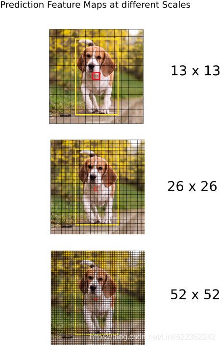

    The authors report that this helps YOLO v3 get better at detecting small objects, a frequent complaint with the earlier versions of YOLO. Upsampling can help the network learn fine-grained features which are instrumental for detecting small objects.

More bounding boxes per image and Output Processing

     For an input image of same size, YOLO v3 predicts more bounding boxes than YOLO v2. For instance, at it’s native resolution of 416 x 416, YOLO v2 predicted 13 x 13 x 5 = 845 boxes. At each grid cell, 5 boxes were detected using 5 anchors.

     On the other hand YOLO v3 predicts boxes at 3 different scales. For an image of size 416 x 416, YOLO predicts ((52 x 52) + (26 x 26) + 13 x 13)) x 3 = 10647 bounding boxes. However, in case of our image, there's only one object, a dog. How do we reduce the detections from 10647 to 1?

     This means that YOLO v3 predicts 10x the number of boxes predicted by YOLO v2. You could easily imagine why it’s slower than YOLO v2. At each scale, every grid can predict 3 boxes using 3 anchors. Since there are three scales, the number of anchor boxes used in total are 9, 3 for each scale.

Thresholding by Object Confidence

     First, we filter boxes based on their objectness score. Generally, boxes having scores below a threshold are ignored.

Non-maximum Suppression非最大抑制

     NMS intends to cure the problem of multiple detections of the same image. For example, all the 3 bounding boxes of the red grid cell may detect a box or the adjacent cells may detect the same object.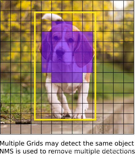

Bounding-box regressionhttps://arxiv.org/pdf/1311.2524.pdf
 be replaced with

小结

YOLO3借鉴了残差网络结构，形成更深的网络层次，以及多尺度检测，提升了mAP及小物体检测效果。如果采用COCO mAP50做评估指标（不是太介意预测框的准确性的话），YOLO3的表现相当惊人，如下图所示，在精确度相当的情况下，YOLOv3的速度是其它模型的3、4倍。

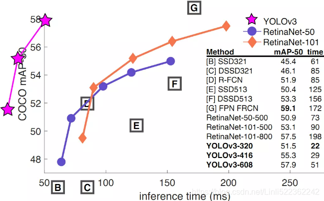
https://towardsdatascience.com/review-yolov3-you-only-look-once-object-detection-eab75d7a1ba6

code:
https://github.com/qqwweee/keras-yolo3

https://machinelearningmastery.com/how-to-perform-object-detection-with-yolov3-in-keras/

https://github.com/allanzelener/YAD2K

https://github.com/xiaochus/YOLOv3

https://github.com/xiaochus

####################################################################################
     The blue box below is the predicted bounding box(predicted ground-truth box) and the dotted rectangle is the anchor box(bounding box priors).
<== <==

     YOLOv3’s architecture is quite similar to the one we just discussed, but with a few important differences:

• It outputs five bounding boxes for each grid cell (instead of just one), and each bounding box comes with an objectness score. It also outputs 20 class probabilities per grid cell, as it was trained on the PASCAL VOC dataset, which contains 20 classes. That’s a total of 145(=5x(4+5+20) ) numbers per grid cell: 5 bounding boxes, each with 4 coordinates, plus 5 objectness scores, plus 20 class probabilities.
   
• Instead of predicting the absolute coordinates of the bounding box centers, YOLOv3 predicts an offset relative to the coordinates of the grid cell, where (0, 0) means the top left of that cell and (1, 1) means the bottom right. For each grid cell, YOLOv3 is trained to predict only bounding boxes whose center lies in that cell (but the bounding box itself generally extends well beyond the grid cell). YOLOv3 applies the logistic sigmoid activation function 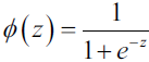to the bounding box coordinatesto ensure they remain in the 0 to 1 range.
• Before training the neural net, YOLOv3 finds five representative bounding box dimensions, called anchor boxes (or bounding box priors). It does this by applying the K-Means algorithm (see Chapter 9) to the height and width of the training set bounding boxes. For example, if the training images contain many pedestrians行人, then one of the anchor boxes will likely have the dimensions of a typical pedestrian. Then when the neural net predicts five bounding boxes per grid cell, it actually predicts how much to rescale each of the anchor boxes. For example, suppose one anchor box(bounding box priors) is 100 pixels tall and 50 pixels wide, and the network predicts, say, a vertical rescaling factor of 1.5 and a horizontal rescaling of 0.9 (for one of the grid cells). This will result in a predicted bounding box of size 150 × 45 pixels(predicted ground-truth box). To be more precise, for each grid cell and each anchor box, the network predicts the log of the vertical and horizontal rescaling factors. Having these priors makes the network more likely to predict bounding boxes of the appropriate dimensions, and it also speeds up training because it will more quickly learn what reasonable bounding boxes look like.
   
• The network is trained using images of different scales: every few batches during training, the network randomly chooses a new image dimension (from 330 × 330 to 608 × 608 pixels). This allows the network to learn to detect objects at different scales. Moreover, it makes it possible to use YOLOv3 at different scales: the smaller scale will be less accurate but faster than the larger scale, so you can choose the right trade-off for your use case.

     There are a few more innovations you might be interested in, such as the use of skip connections to recover some of the spatial resolution that is lost in the CNN (we will discuss this shortly, when we look at semantic segmentation). In the 2016 paper, the authors introduce the YOLO9000 model that uses hierarchical classification: the model predicts a probability for each node in a visual hierarchy called WordTree. This makes it possible for the network to predict with high confidence that an image represents, say, a dog, even though it is unsure what specific type of dog. I encourage you to go ahead and read all three papers: they are quite pleasant to read, and they provide excellent examples of how Deep Learning systems can be incrementally improved.

Mean Average Precision (mAP)

P(positive): Your Target,             N(negative): not your target
TP : Oject(Your Target) ==> are correctly(True) predicted as positive(Your Target ==> Your Target)
TN : Oject(Not Your Target) ==> are correctly(True) predicted as negative(not your target==>not your target)
FP : Oject(Not Your Target) ==> are incorrectly(False) predicted as positive(not your target==>Your Target)
FN: Oject(Your Target) ==>are incorrectly(False) predicted as negative(your target==>not your target)

     A very common metric used in object detection tasks is the mean Average Precision (mAP). “Mean Average” sounds a bit redundant, doesn’t it? To understand this metric, let’s go back to two classification metrics we discussed in Chapter 3:

• precision( Precision = TP/(TP+FP) # True predicted/ (True predicted + False predicted); Precision answers the following: How many of those who we labeled as diabetic(target) are actually diabetic?) and
• recall(aka Sensitivity, Recall = TP/(TP+FN, detected objects are your target), Of all the people who are diabetic(target), how many of those we correctly predict?). Remember the trade-off:the higher the recall, the lower the precision. You can visualize this in a precision/recall curve (see Figure 3-5).To summarize this curve into a single number, we could compute its area under the curve (AUC, sklearn.metrics.roc_auc_score(). https://blog.csdn.net/Linli522362242/article/details/103786116

 you should prefer the PR curve whenever the positive class(target) is rare or when you care more about the false positives than the false negatives, and the ROC curve otherwise. for example,  a credit card company wants to release a credict card to regular customer(target), but you will care about FP( incorrectly classified some customer have default records违约记录 as regular customer)

# 03_Classification_import name fetch_mldata_cross_val_plot_digits_ML_Project Checklist_confusion matr
# https://blog.csdn.net/Linli522362242/article/details/103786116
y_train_5 = (y_train==5)
sgd_clf = SGDClassifier(random_state=42, max_iter=1000, tol=1e-3)
#cv : int, cross-validation generator or an iterable, default=None
#     to specify the number of folds in a (Stratified)KFold,
y_decision_scores = cross_val_predict(sgd_clf, X_train, y_train_5, cv=3, method="decision_function")

sklearn.metrics.roc_auc_score(y_train_5, y_decision_scores)

precisions, recalls, thresholds = precision_recall_curve(y_train_5, y_decision_scores)

     But note that the precision/recall curve may contain a few sections where precision actually goes up when recall increases, especially at low recall values (you can see this at the top left of Figure 3-5). This is one of the motivations for the mAP metric.

Mean Average Precision (mAP)

import numpy as np
import matplotlib.pyplot as plt

def maximum_precisions(precisions):
  # precisions = [0.91, 0.94, 0.96, 0.94, 0.95, 0.92, 0.80, 0.60, 0.45, 0.20, 0.10]
  # np.flip( precisions )
  #    array([0.1 , 0.2 , 0.45, 0.6 , 0.8 , 0.92, 0.95, 0.94, 0.96, 0.94, 0.91])
  # np.maximum.accumulate( np.flip(precisions) )
  #    array([0.1 , 0.2 , 0.45, 0.6 , 0.8 , 0.92, 0.95, 0.95, 0.96, 0.96, 0.96])
  # np.flip( np.maximum.accumulate( np.flip(precisions) ) )
  #    array([0.96, 0.96, 0.96, 0.95, 0.95, 0.92, 0.8 , 0.6 , 0.45, 0.2 , 0.1 ])
  return np.flip( np.maximum.accumulate( np.flip(precisions) ) )

recall(aka Sensitivity, Recall = TP/(TP+FN, detected objects are your target), Of all the people who are diabetic(target), how many of those we correctly predict?).

recalls = np.linspace(0,1,11)

precisions = [0.91, 0.94, 0.96, 0.94, 0.95, 0.92, 0.80, 0.60, 0.45, 0.20, 0.10]
max_precisions = maximum_precisions(precisions)
#      array([0.96, 0.96, 0.96, 0.95, 0.95, 0.92, 0.8 , 0.6 , 0.45, 0.2 , 0.1 ])
mAP = max_precisions.mean()

plt.plot(recalls, precisions, 'yo--', label='Precision')
plt.plot(recalls, max_precisions, 'bo-', label='Max Precision')
plt.plot([0,1], [mAP, mAP], 'k:', linewidth=3, label='mAP')

plt.xlabel('Recall')
plt.ylabel('Precision')
plt.grid(True)
plt.axis( [0,1, 0,1] )
plt.legend( loc='lower center', fontsize=14)

plt.show()

 

     Suppose the classifier has 90% precision at 10% recall, but 96% precision at 20% recall. There’s really no trade-off here: it simply makes more sense to use the classifier at 20% recall rather than at 10% recall, as you will get both higher recall and higher precision. So instead of looking at the precision at 10% recall, we should really be looking at the maximum precision that the classifier can offer with at least 10% recall. It would be 96%, not 90%. Therefore, one way to get a fair idea of the model’s performance is to compute the maximum precision you can get with at least 0% recall, then 10% recall, 20%, and so on up to 100%, and then calculate the mean of these maximum precisions. This is called the Average Precision (AP) metric. Now when there are more than two classes, we can compute the AP for each class, and then compute the mean AP (mAP). That’s it!

     In an object detection system, there is an additional level of complexity: what if the system detected the correct class, but at the wrong location (i.e., the bounding box is completely off)? Surely we should not count this as a positive prediction. One approach is to define an IOU threshold: for example, we may consider that a prediction is correct only if the IOU is greater than, say, 0.5, and the predicted class is correct. The corresponding mAP is generally noted [email protected] (or mAP@50%, or sometimes just AP50). In some competitions (such as the PASCAL VOC challenge), this is what is done. In others (such as the COCO competition), the mAP is computed for different IOU thresholds (0.50, 0.55, 0.60, …, 0.95), and the final metric is the mean of all these mAPs (noted AP@[.50:.95] or AP@[.50:0.05:.95]). Yes, that’s a mean mean average.

     Several YOLO implementations built using TensorFlow are available on GitHub. In particular, check out Zihao Zang’s TensorFlow 2 implementationhttps://github.com/zzh8829/yolov3-tf2. Other object detection models are available in the TensorFlow Models project, many with pretrained weights; and some have even been ported to TF Hub, such as SSD31 and Faster-RCNN,32 which are both quite popular. SSD is also a “single shot” detection model, similar to YOLO. Faster R-CNN is more complex: the image first goes through a CNN, then the output is passed to a Region Proposal Network (RPN) that proposes bounding boxes that are most likely to contain an object, and a classifier is run for each bounding box, based on the cropped output of the CNN.

     The choice of detection system depends on many factors: speed, accuracy, available pretrained models, training time, complexity, etc. The papers contain tables of metrics, but there is quite a lot of variability in the testing environments, and the technologies evolve so fast that it is difficult to make a fair comparison that will be useful for most people and remain valid for more than a few months.

     So, we can locate objects by drawing bounding boxes around them. Great! But perhaps you want to be a bit more precise. Let’s see how to go down to the pixel level.

bilinear interpolation

线性插值

先讲一下线性插值：已知数据 (x0, y0) 与 (x1, y1)，要计算 [x0, x1] 区间内某一位置 x 在直线上的y值: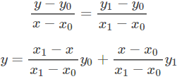 

仔细看就是用x和x0，x1的距离作为一个权重，用于y0和y1的加权。双线性插值本质上就是在两个方向上做线性插值。

     In mathematics, bilinear interpolation is an extension of linear interpolation for interpolating functions of two variables (e.g., x and y) on a rectilinear 2D grid.

     Bilinear interpolation is performed using linear interpolation first in one direction, and then again in the other direction. Although each step is linear in the sampled values and in the position, the interpolation as a whole is not linear but rather quadratic in the sample location.

     Bilinear interpolation is one of the basic resampling techniques in computer vision and image processing, where it is also called bilinear filtering or bilinear texture mapping双线性滤波或双线性纹理映射.

bilinear interpolation

https://en.wikipedia.org/wiki/Bilinear_interpolation
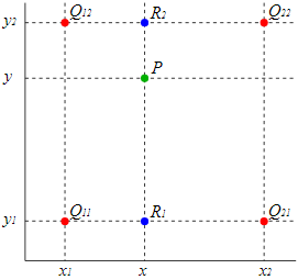
     Suppose that we want to find the value of the unknown function f at the point P(x, y). It is assumed that we know the value of f at the four points Q11 = (x1, y1), Q12 = (x1, y2), Q21 = (x2, y1), and Q22 = (x2, y2).

     We first do linear interpolation in the x-direction. This yields 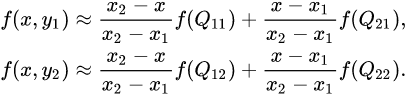and  , 

     We proceed by interpolating in the y-direction to obtain the desired estimate:

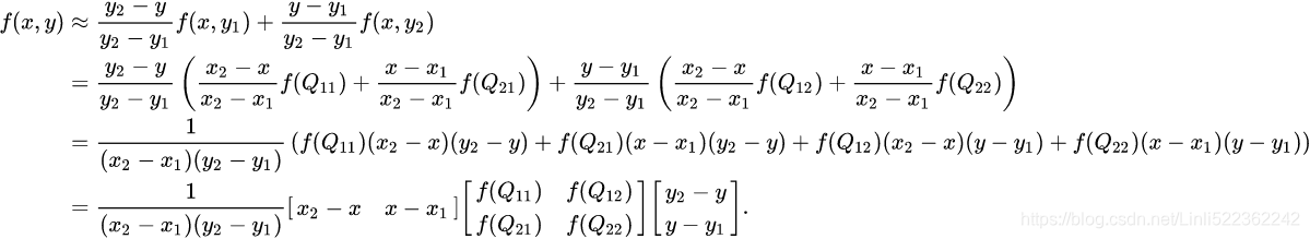
Note that we will arrive at the same result if the interpolation is done first along the y direction and then along the x direction

Alternative algorithm

 VS svd https://blog.csdn.net/Linli522362242/article/details/105139547

An alternative way to write the solution to the interpolation problem is 
where the coefficients are found by solving the linear system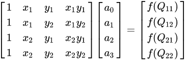 

yielding the result 

If a solution is preferred in terms of f(Q), then we can write 

where the coefficients are found by calculating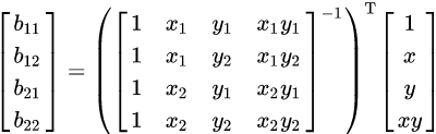 

Unit square

     If we choose a coordinate system in which the four points where f is known are Q11=(x1, y1)=(0, 0), Q21=(x2, y1)=(1, 0), Q12=(x1, y2)=(0, 1), and Q22=(x2, y2)=(1, 1), then the interpolation formula simplifies to 
or equivalently, in matrix operations: 

Application in image processing

     In computer vision and image processing, bilinear interpolation is used to resample images and textures. An algorithm is used to map a screen pixel location to a corresponding point on the texture map. A weighted average of the attributes (color, transparency, etc.) of the four surrounding texels周围的四个纹理 is computed and applied to the screen pixel. This process is repeated for each pixel forming the object being textured.

     When an image needs to be scaled up, each pixel of the original image needs to be moved in a certain direction based on the scale constant. However, when scaling up an image by a non-integral scale factor, there are pixels (i.e., holes) that are not assigned appropriate pixel values. In this case, those holes should be assigned appropriate RGB or grayscale values so that the output image does not have non-valued pixels.

     Bilinear interpolation can be used where perfect image transformation with pixel matching is impossible, so that one can calculate and assign appropriate intensity values to pixels. Unlike other interpolation techniques such as nearest-neighbor interpolation and bicubic interpolation, bilinear interpolation uses values of only the 4 nearest pixels, located in diagonal directions from a given pixel, in order to find the appropriate color intensity values of that pixel.
Comparison of bilinear interpolation with some 1- and 2-dimensional interpolations. Black and red/yellow/green/blue dots correspond to the interpolated point and neighbouring samples, respectively. Their heights above the ground correspond to their values.

     Bilinear interpolation considers the closest 2 × 2 neighborhood of known pixel values surrounding the unknown pixel's computed location. It then takes a weighted average of these 4 pixels to arrive at its final, interpolated value.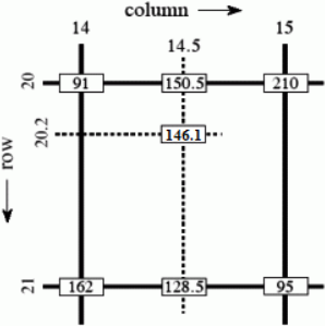
As seen in the example on the right, the intensity value at the pixel computed to be at row 20.2, column 14.5 can be calculated by first linearly interpolating between the values at column 14 and 15 on each rows 20 and 21, giving
<==

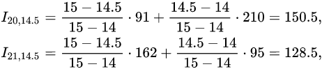and then interpolating linearly between these values, giving
 <==

     This algorithm reduces some of the visual distortion caused by resizing an image to a non-integral zoom factor, as opposed to nearest-neighbor interpolation, which will make some pixels appear larger than others in the resized image.

Semantic Segmentation

     In semantic segmentation, each pixel is classified according to the class of the object it belongs to (e.g., road, car, pedestrian[pəˈdestriən], building, etc.), as shown in Figure 14-26. Note that different objects of the same class are not distinguished. For example, all the bicycles on the right side of the segmented image end up as one big lump块 of pixels. The main difficulty in this task is that when images go through a regular CNN, they gradually lose their spatial resolution (due to the layers with strides greater than 1); so, a regular CNN may end up knowing that there’s a person somewhere in the bottom left of the image, but it will not be much more precise than that.
Figure 14-26. Semantic segmentation

     Just like for object detection, there are many different approaches to tackle this problem, some quite complex. However, a fairly simple solution was proposed in the 2015 paper by Jonathan Long et al. we discussed earlier. The authors start by taking a pretrained CNN and turning it into an FCN. The CNN applies an overall stride of 32 to the input image (i.e., if you add up all the strides greater than 1), meaning the last layer outputs feature maps that are 32 times smaller than the input image. This is clearly too coarse粗糙, so they add a single upsampling layer that multiplies the resolution by 32.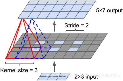
Figure 14-27. Upsampling using a transposed convolutional layer

# Upscaled Image
stride = 2, kernel size=3
(height-1)*stride + 2*kernel_size-1, # e.g. (3-1)*2 + 2*3 -1 = 9
(width-1) *stride + 2*kernel_size-1, # e.g. (2-1)*2 + 2*3 -1 = 7

# then assign the original image values to the upscaled image
  upscaled[:, # batches
                 kernel_size-1:(height-1)*stride + kernel_size:stride, # 3-1:(3-1)*2+3:2 ==> 2:7:2
                 kernel_size-1:(width-1) *stride + kernel_size:stride, # 3-1:(2-1)*2+3:2 ==> 2:5:2
                :]=images
# Upsampling using a transposed convolutional layer ==> weights

upscaled = upscale_images(X, stride=2, kernel_size=3)
# conv_transpose = tf.keras.layers.Conv2DTranspose(filters=5, 
#                                                  kernel_size=3,
#                                                  strides=2,
#                                                  padding='VALID')
# output = conv_transpose(X)           # kernel_size=3, kernel_size=3, filters=5, 3 channels=3   
weights, bias = conv_transpose.weights # (3, 3, 5, 3), (5,)
reversed_filters = np.flip( weights.numpy(), axis=[0,1])
reversed_filters = np.transpose(reversed_filters, 
                                [0,1,3,2]) # axis
# reversed_filters.shape # ==> (width=3, height=3, 3 channels, 5 filters)   

### OR

Stride = 2, padding=0 
input_stretched_height =  input_height + (Stride-1) *(input_height-1)   = 3 + (2-1)*(3-1)=5
input_stretched_width   = input_width + (Stride -1) * (input_width -1) = 2 + (2-1)*(2-1)=3

new Stride :  = 1
new padding: max(Input_shape) -padding-1=max(2,3)-0-1=2

perform a regular convolution:
output_height = (5 + 2 * 2 - 3 ) /1 + 1 = 7
output_width  = (3 + 2 * 2 - 3 ) /1 + 1 = 5

Conclution : output_shape == (input_shape-1)*stride - 2*padding+ kernel_size =( [3,2] -1 )*2 - 2*0 + (3,3) =[4,2] - 2*0 + (3,3) = [7,5]

     There are several solutions available for upsampling (increasing the size of an image), such as bilinear interpolation, but that only works reasonably well up to ×4 or ×8. Instead, they use a transposed convolutional layer (This type of layer is sometimes referred to as a deconvolution layer去卷积层, but it does not perform what mathematicians call a deconvolution, so this name should be avoided.):  it is equivalent to

• first stretching the image by inserting empty rows and columns (full of zeros), then
• performing a regular convolution (see Figure 14-27).
• Alternatively, some people prefer to think of it as a regular convolutional layer that uses fractional strides (e.g., 1/2 in Figure 14-27). The transposed convolutional layer can be initialized to perform something close to linear interpolation, but since it is a trainable layer, it will learn to do better during training. In tf.keras, you can use the Conv2DTranspose layer.

     In a transposed convolutional layer, the stride defines how much the input will be stretched, not the size of the filter steps, so the larger the stride, the larger the output (unlike for convolutional layers or pooling layers).

# Transpose convolutions:

import tensorflow as tf
import numpy as np
import matplotlib.pyplot as plt
from sklearn.datasets import load_sample_image

# Load sample images
china = load_sample_image("china.jpg") / 255
flower = load_sample_image("flower.jpg") / 255
images = np.array([china, flower])
# image_height=427 , image_width=640

# https://blog.csdn.net/Linli522362242/article/details/108396485
china_box = [0, 0.03, 1, 0.68] # crop range(positions) in percentages
flower_box = [0.19, 0.26, 0.86, 0.7]
images_resized = tf.image.crop_and_resize(images, 
                                          boxes=[china_box, flower_box], 
                                          box_indices=[0,1], 
                                          crop_size=[224, 224])

def plot_color_image(image):
    plt.imshow(image, interpolation="nearest")
    plt.axis("off")

plot_color_image(images_resized[0])
plt.show()
plot_color_image(images_resized[1])
plt.show()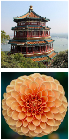

################################# tf.keras.layers.Conv2DTranspose #############################

tf.random.set_seed(42)
X = images_resized.numpy()
# X.shape # (2, 224, 224, 3)

conv_transpose = tf.keras.layers.Conv2DTranspose(filters=5, 
                                                 kernel_size=3,
                                                 strides=2,
                                                 padding='VALID') #p=0
output = conv_transpose(X)
output.shape

 # =(224-1)*2-2*0+3 =449
# without normalization and interpolation='bicubic'

fig = plt.figure( figsize=(12,8) )
gs = mpl.gridspec.GridSpec( nrows=1, ncols=2, width_ratios=[1,2] )

ax1 = fig.add_subplot( gs[0,0] )
ax1.set_title( "Input", fontsize=14 )
ax1.imshow( X[0] )
ax1.axis("off")

ax2 = fig.add_subplot( gs[0,1] )
ax2.set_title( "Output", fontsize=14 )
# 0:  plot the output for the 1st image
ax2.imshow(  output[0, ..., :3] )
ax2.axis("off")

plt.show()

 
#  normalization 

import matplotlib as mpl

def normalize(X):
  return ( X-tf.reduce_min(X) ) / ( tf.reduce_max(X) - tf.reduce_min(X) )

fig = plt.figure( figsize=(12,8) )
gs = mpl.gridspec.GridSpec( nrows=1, ncols=2, width_ratios=[1,2] )

ax1 = fig.add_subplot( gs[0,0] )
ax1.set_title( "Input", fontsize=14 )
ax1.imshow( X[0] )
ax1.axis("off")

ax2 = fig.add_subplot( gs[0,1] )
ax2.set_title( "Output", fontsize=14 )
# 0:  plot the output for the 1st image
ax2.imshow(  normalize( output[0, ..., :3] ) )
ax2.axis("off")

plt.show()

 

normalization and interpolation='bicubic'

import matplotlib as mpl

def normalize(X):
  return ( X-tf.reduce_min(X) ) / ( tf.reduce_max(X) - tf.reduce_min(X) )

fig = plt.figure( figsize=(12,8) )
gs = mpl.gridspec.GridSpec( nrows=1, ncols=2, width_ratios=[1,2] )

ax1 = fig.add_subplot( gs[0,0] )
ax1.set_title( "Input", fontsize=14 )
ax1.imshow( X[0] )
ax1.axis("off")

ax2 = fig.add_subplot( gs[0,1] )
ax2.set_title( "Output", fontsize=14 )
# 0:  plot the output for the 1st image  # 3 ==>bicubic
ax2.imshow( normalize( output[0, ..., :3] ), interpolation='bicubic')
ax2.axis("off")

plt.show()

################ np.flip https://numpy.org/doc/stable/reference/generated/numpy.flip.html

A = np.arange(8).reshape((2,2,2))
A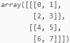

 

np.flip(A, 0)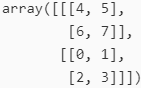

 

np.flip(A, (0, 2))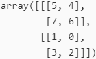

 

################

# Upscaled Image

################################# tf.nn.conv2d #############################

(batch_size, height, width, channels)

def upscale_images( images, stride, kernel_size ):
  # (2, 224, 224, 3)
  batch_size, height, width, channels = images.shape
  upscaled = np.zeros( ( batch_size,
                         (height-1)*stride + 2*kernel_size-1, # e.g. (3-1)*2 + 2*3 -1 = 9
                         (width-1) *stride + 2*kernel_size-1, # e.g. (2-1)*2 + 2*3 -1 = 7
                         channels
                       ) )
  upscaled[:,
           kernel_size-1:(height-1)*stride + kernel_size:stride, # 3-1:(3-1)*2+3:2 ==> 2:7:2
           kernel_size-1:(width-1) *stride + kernel_size:stride, # 3-1:(2-1)*2+3:2 ==> 2:5:2
           :]=images
  return upscaled

# Upsampling using a transposed convolutional layer ==> weights 

upscaled = upscale_images(X, stride=2, kernel_size=3)
# conv_transpose = tf.keras.layers.Conv2DTranspose(filters=5, 
#                                                  kernel_size=3,
#                                                  strides=2,
#                                                  padding='VALID')
# output = conv_transpose(X)           # kernel_size=3, kernel_size=3, filters=5, 3 channels=3   
weights, bias = conv_transpose.weights # (3, 3, 5, 3), (5,) 
# w_m,...,w2,w1,w0= b # so we need to filp weight
reversed_filters = np.flip( weights.numpy(), axis=[0,1]) 
reversed_filters = np.transpose(reversed_filters, 
                                [0,1,3,2]) # axis
# reversed_filters.shape # ==> (width=3, height=3, 3 channels, 5 filters) 

# performing a regular convolution and new Stride :  = 1 + upscaled image and  reversed_filters

manual_output = tf.nn.conv2d( upscaled, 
                             reversed_filters, 
                             strides=1, 
                             padding='VALID')
manual_output.shape

def normalize(X):
  return ( X-tf.reduce_min(X) ) / ( tf.reduce_max(X) - tf.reduce_min(X) )

fig = plt.figure( figsize=(12,8) )
gs = mpl.gridspec.GridSpec( nrows=1, ncols=3, width_ratios=[1,2,2])

ax1 = fig.add_subplot( gs[0,0] )
ax1.set_title("Input", fontsize=14)
ax1.imshow(X[0]) # plot the 1st image
ax1.axis("off")

ax2 = fig.add_subplot( gs[0,1] )
ax2.set_title("Upscaled", fontsize=14)
ax2.imshow(upscaled[0], interpolation="bicubic")
ax2.axis("off")

ax3 = fig.add_subplot( gs[0,2] )
ax3.set_title("Output", fontsize=14)
ax3.imshow( normalize(manual_output[0, ..., :3]), interpolation="bicubic" )
ax3.axis("off")

plt.show()

np.allclose( output, manual_output.numpy(), atol=1e-7)

 # so the results from  tf.keras.layers.Conv2DTranspose and tf.nn.conv2d are equal
############################################

TensorFlow Convolution Operations

TensorFlow also offers a few other kinds of convolutional layers:

• keras.layers.Conv1D
       Creates a convolutional layer for 1D inputs, such as time series or text (sequences of letters or words), as we will see in Chapter 15.
• keras.layers.Conv3D
       Creates a convolutional layer for 3D inputs, such as 3D PET scans.
• dilation_rate膨胀率[daɪ'leɪʃn]
       Setting the dilation_rate hyperparameter of any convolutional layer to a value of 2 or more creates an à-trous convolutional layer (“à trous” is French for “with holes”). This is equivalent to using a regular convolutional layer with a filter dilated by inserting rows and columns of zeros (i.e., holes). For example, a 1 × 3 filter equal to [[1,2,3]] may be dilated with a dilation rate of 4, resulting in a dilated filter of [[1, 0, 0, 0, 2, 0, 0, 0, 3]]. This lets the convolutional layer have a larger receptive field at no computational price and using no extra parameters.
  dilation_filter_dimension =dilation_rate * ( original_filter_dimensions - 1 ) + 1 = 4 *( [1,3] -1) + 1 = 4*[0,2]+1 = [0,8]+1=[1,9]
• tf.nn.depthwise_conv2d()
       Can be used to create a depthwise convolutional layer (but you need to create the variables yourself). It applies every filter to every individual input channel independently. Thus, if there are fn filters and fn′ input channels, then this will output fn × fn′ feature maps.

############################################
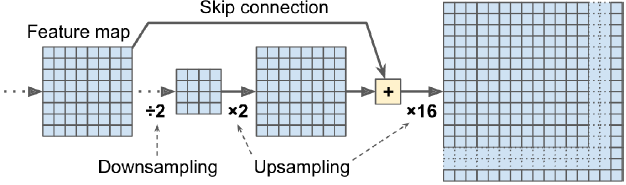Figure 14-28. Skip layers recover some spatial resolution from lower layers

     This solution is OK, but still too imprecise. To do better, the authors added skip connections from lower layers: for example, they upsampled the output image by a factor of 2 (instead of 32), and they added the output of a lower layer that had this double resolution. Then they upsampled the result(after + operation) by a factor of 16, leading to a total upsampling factor of 32 (see Figure 14-28). This recovered some of the spatial resolution that was lost in earlier pooling layers. In their best architecture, they used a second similar skip connection to recover even finer details from an even lower layer. In short, the output of the original CNN goes through the following extra steps: upscale ×2, add the output of a lower layer (of the appropriate scale), upscale ×2, add the output of an even lower layer, and finally upscale ×8. It is even possible to scale up beyond the size of the original image: this can be used to increase the resolution of an image, which is a technique called super-resolution.

     Once again, many GitHub repositories provide TensorFlow implementations of semantic segmentation (TensorFlow 1 for now), and you will even find pretrained instance segmentation models in the TensorFlow Models project. Instance segmentation is similar to semantic segmentation, but instead of merging all objects of the same class into one big lump, each object is distinguished from the others (e.g., it identifies each individual bicycle). At present, the instance segmentation models available in the TensorFlow Models project are based on the Mask R-CNN architecture, which was proposed in a 2017 paper(Kaiming He et al., “Mask R-CNN,” arXiv preprint arXiv:1703.06870 (2017).): it extends the Faster R-CNN model by additionally producing a pixel mask for each bounding box. So not only do you get a bounding box around each object, with a set of estimated class probabilities, but you also get a pixel mask that locates pixels in the bounding box that belong to the object.

     As you can see, the field of Deep Computer Vision is vast and moving fast, with all sorts of architectures popping out every year, all based on convolutional neural networks.
The progress made in just a few years has been astounding[ əˈstaʊndɪŋ]使人震惊的, and researchers are now focusing on harder and harder problems, such as adversarial learning (which attempts to make the network more resistant to images designed to fool it), explainability (understanding why the network makes a specific classification), realistic image generation (which we will come back to in Chapter 17), and single-shot learning (a system that can recognize an object after it has seen it just once). Some even explore completely novel architectures, such as Geoffrey Hinton’s capsule networks (Geoffrey Hinton et al., “Matrix Capsules with EM Routing,” Proceedings of the International Conference on Learning Representations (2018).). Now on to the next chapter, where we will look at how to process sequential data such as time series using recurrent neural networks and convolutional neural networks.

Exercises

https://blog.csdn.net/Linli522362242/article/details/114817809