The batter[ˈbætər]击球员 hits the ball. The outfielder[ˈaʊtfi:ldə(r)]外场手 immediately starts running, anticipating the ball’s trajectory[trəˈdʒektəri]轨线. He tracks it, adapts his movements, and finally catches it (under a thunder of applause). Predicting the future is something you do all the time, whether you are finishing a friend’s sentence or anticipating the smell of coffee at breakfast. In this chapter we will discuss recurrent neural networks (RNNs), a class of nets that can predict the future (well, up to a point, of course). They can analyze time series data such as stock prices, and tell you when to buy or sell. In autonomous driving systems, they can anticipate car trajectories and help avoid accidents. More generally, they can work on sequences of arbitrary lengths, rather than on fixed-sized inputs like all the nets we have considered so far. For example, they can take sentences, documents, or audio samples as input, making them extremely useful for natural language processing(NLP) applications such as automatic translation or speech-to-text, or sentiment analysis (e.g., reading movie reviews and extracting the rater’s feeling about the movie).

In this chapter we will first look at the fundamental concepts underlying RNNs and how to train them using backpropagation through time, then we will use them to
forecast a time series. After that we’ll explore the two main difficulties that RNNs face:

• Unstable gradients (discussed in Chapter 11, e.g. vanishing/exploding gradients), which can be alleviated using various techniques, including recurrent dropout and recurrent layer normalization
• A (very) limited short-term memory, which can be extended using LSTM and GRU cells

RNNs are not the only types of neural networks capable of handling sequential data: for small sequences, a regular dense network can do the trick; and for very long
sequences, such as audio samples or text, convolutional neural networks can actually work quite well too. We will discuss both of these possibilities, and we will finish this
chapter by implementing a WaveNet: this is a CNN architecture capable of handling sequences of tens of thousands of time steps. In Chapter 16, we will continue to
explore RNNs and see how to use them for natural language processing(NLP), along with more recent architectures based on attention mechanisms. Let’s get started!

Recurrent Neurons and Layers

Up to now we have focused on feedforward neural networks, where the activations flow only in one direction, from the input layer to the output layer (a few exceptions
are discussed in Appendix E). A recurrent neural network looks very much like a feedforward neural network, except it also has connections pointing backward. Let’s
look at the simplest possible RNN, composed of one neuron receiving inputs, producing an output, and sending that output back to itself, as shown in Figure 15-1
(left). At each time step t (also called a frame帧), this recurrent neuron receives the inputs as well as its own output from the previous time step, . Since there is no previous output at the first time step, it is generally set to 0. We can represent this tiny network against the time axis, as shown in Figure 15-1 (right). This is called unrolling the network through time随着时间的推移展开网络 (it’s the same recurrent neuron represented once per time step).
Figure 15-1. A recurrent neuron (left) unrolled through time (right)

You can easily create a layer of recurrent neurons. At each time step t, every neuron
(###
If the input received by the recurrent neuron is a vector, then the recurrent neuron should be a neuron containing multiple units.
If the input received by the recurrent neuron is a scalar, then the recurrent neuron is just a neuron of one unit.
###)
receives both the input vector
(###
At time step t, the input instance contains multiple features, and each neuron receives multiple features
###)
and the output vector from the previous time step , as shown in Figure 15-2. Note that both the inputs and outputs are vectors now (when there was just a single neuron, the output was a scalar. A scalar is a single number, usually represented by a lowercase variable name).
Figure 15-2. A layer of recurrent neurons (left) unrolled through time (right)

Each recurrent neuron has two sets of weights: one for the inputs and the other for the outputs of the previous time step, . Let’s call these weight vectors and . If we consider the whole recurrent layer instead of just one recurrent neuron, we can place all the weight vectors in two weight matrices,
(###
shape = [num_input_instances=len(recurrent output neurons), num_features_for_each_instance=len(weight vectors) ]
###)

and . The output vector of the whole recurrent layer can then be computed pretty much as you might expect, as shown in Equation 15-1 ( is the bias vector and ϕ(·) is the activation function (e.g., ReLU).

Equation 15-1. Output of a recurrent layer for a single instance
### note: contains just one instance with multiple features per time step t and is just one item ###

Just as with feedforward neural networks, we can compute a recurrent layer’s output in one shot for a whole mini-batch by placing all the inputs at time step t in an input matrix (see Equation 15-2).

Equation 15-2. Outputs of a layer of recurrent neurons for all instances in a minibatch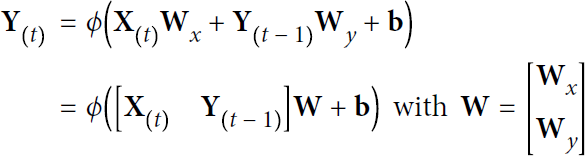
### note: contains multiple instances with multiple features per time step t ###

In this equation:

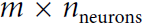• is an matrix containing the layer’s outputs at time step t for each instance in the mini-batch (m is the number of instances in the mini-batch and is the number output of neurons).
• is an matrix containing the inputs for all instances (is the number of input features).
• is an matrix containing the connection weights for the inputs of the current time step.
• is an matrix containing the connection weights for the outputs of the previous time step.
• is a vector of size containing each output neuron’s bias term.
• The weight matrices and are often concatenated vertically into a single weight matrix of shape 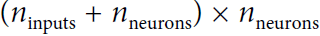(see the second line of Equation 15-2).
• The notation represents the horizontal concatenation of the matrices and .

Notice that is a function of and , which is a function of and , which is a function of and , and so on. This makes a function of all the inputs since time t = 0 (that is, ). At the first time step, t = 0, there are no previous outputs, so they are typically assumed to be all zeros.
######################################### https://blog.csdn.net/Linli522362242/article/details/113846940

• The weight matrices and are often concatenated horizontally into a single weight matrix of shape (see the second line of Equation 15-2).
• The notation represents the vertical concatenation of the matrices and .
==> , ==>, ==>

the same weights are used at every time step
#########################################

Memory Cells

Since the output of a recurrent neuron at time step t is a function of all the inputs from previous time steps, you could say it has a form of memory. A part of a neural network that preserves some state across time steps is called a memory cell (or simply a cell). A single recurrent neuron, or a layer of recurrent neurons, is a very basic cell, capable of learning only short patterns (typically about 10 steps long, but this varies depending on the task). Later in this chapter, we will look at some more complex and powerful types of cells capable of learning longer patterns (roughly 10 times longer, but again, this depends on the task).

In general a cell’s state at time step t, denoted (the “h” stands for “hidden”), is a function of some inputs at that time step and its state at the previous time step: = . Its output at time step t, denoted , is also a function of the previous state and the current inputs. In the case of the basic cells we have discussed so far, the output is simply equal to the state, but in more complex cells this is not always the case, as shown in Figure 15-3.
Figure 15-3. A cell’s hidden state and its output may be different

Input and Output Sequences

An RNN can simultaneously take a sequence of inputs and produce a sequence of outputs (see the top-left network in Figure 15-4). This type of sequence-to-sequence network
（### Many-to-many: Both the input and output arrays are sequences. This category can be further divided based on whether the input and output are synchronize['sɪŋkrənaɪzd]同步的.

An example of a synchronized many-to-many modeling task is video classification, where each frame in a video is labeled.
An example of a delayed many-to-many modeling task would be translating one language into another. For instance, an entire English sentence must be read and processed by a machine before its translation into German is produced.

###） is useful for predicting time series such as stock prices: you feed it the prices over the last N days, and it must output the prices shifted by one day into the future (i.e., from N – 1 days ago to tomorrow). https://blog.csdn.net/Linli522362242/article/details/113846940
VSFigure 15-4. Seq-to-seq (top left), seq-to-vector (top right), vector-to-seq (bottom left), and Encoder–Decoder (bottom right) networks

Alternatively, you could feed the network a sequence of inputs and ignore all outputs except for the last one (see the top-right network in Figure 15-4). In other words, this is a sequence-to-vector network
（### Many-to-one: The input data is a sequence, but the output is a fixed-size vector or scalar, not a sequence. For example, in sentiment analysis, the input is text-based (for example, a movie review) and the output is a class label (for example, a label denoting whether a reviewer liked the movie).
###）. For example, you could feed the network a sequence of words corresponding to a movie review, and the network would output a sentiment score (e.g., from –1 [hate] to +1 [love]).

Conversely, you could feed the network the same input vector over and over again at each time step and let it output a sequence (see the bottom-left network of Figure 15-4
（### One-to-many: The input data is in standard format and not a sequence, but the output is a sequence. An example of this category is image captioning—the input is an image and the output is an English phrase summarizing the content of that image)
###）. This is a vector-to-sequence network. For example, the input could be an image (or the output of a CNN), and the output could be a caption for that image.

Lastly, you could have a sequence-to-vector network, called an encoder, followed by a vector-to-sequence network, called a decoder (see the bottom-right network of Figure 15-4). For example, this could be used for translating a sentence from one language to another. You would feed the network a sentence in one language, the encoder would convert this sentence into a single vector representation, and then the decoder would decode this vector into a sentence in another language. This two-step model, called an Encoder–Decoder, works much better than trying to translate on the fly with a single sequence-to-sequence RNN (like the one represented at the top left): the last words of a sentence can affect the first words of the translation, so you need to wait until you have seen the whole sentence before translating it. We will see how to implement an Encoder–Decoder in Chapter 16 (as we will see, it is a bit more complex than in Figure 15-4 suggests).

Sounds promising, but how do you train a recurrent neural network?

Training RNNs

To train an RNN, the trick is to unroll it through time (like we just did) and then simply use regular backpropagation (see Figure 15-5). This strategy is called backpropagation through time (BPTT).
Figure 15-5. Backpropagation through time

Just like in regular backpropagation,

there is a first forward pass through the unrolled network (represented by the dashed arrows).
Then the output sequence is evaluated using a cost function (where T is the max time step). Note that this cost function may ignore some outputs, as shown in Figure 15-5 (for example, in a sequence-to-vector RNN, all outputs are ignored except for the very last one).
The gradients of that cost function are then propagated backward through the unrolled network (represented by the solid arrows).
Finally the model parameters are updated using the gradients computed during BPTT.

Note that the gradients flow backward through all the outputs used by the cost function, not just through the final output (for example, in Figure 15-5 the cost function is computed using the last three outputs of the network, , and , so gradients flow through these three outputs, but not through and ). Moreover, since the same parameters W and b are used at each time step, backpropagation will do the right thing and sum over all time steps.

Fortunately, tf.keras takes care of all of this complexity for you—so let’s start coding!

Forecasting a Time Series

Suppose you are studying the number of active users per hour on your website, or the daily temperature in your city, or your company’s financial health, measured quarterly using multiple metrics. In all these cases, the data will be a sequence of one or more values per time step. This is called a time series. In the first two examples there is a single value per time step, so these are univariate time series, while in the financial example there are multiple values per time step (e.g., the company’s revenue, debt, and so on), so it is a multivariate time series. A typical task is to predict future values, which is called forecasting. Another common task is to fill in the blanks: to predict (or rather “postdict”) missing values from the past. This is called imputation. For example, Figure 15-6 shows 3 univariate time series, each of them 50 time steps long, and the goal here is to forecast the value at the next time step (represented by the X) for each of them.
Figure 15-6. Time series forecasting

For simplicity, we are using a time series generated by the generate_time_series() function, shown here:

import numpy as np

def generate_time_series(batch_size, n_steps):
    freq1, freq2, offsets1, offsets2 = np.random.rand(4, batch_size, 1)
    # print(freq1.shape) # (batches,1)
    time = np.linspace(0,1, n_steps) 
    # print(time.shape)  # (n_steps,)
    
    # https://numpy.org/doc/stable/user/basics.broadcasting.html
    # time-offsets1 shape: (n_steps,)-(batches,1) 
    # the axes operation is from right to left : 
    #                         time.shape(n_steps,)         - freq1.shape(batches,1)
    #                      ==>time.shape(,n_steps)         - freq1.shape(batches,1)
    # broadcast operation  ==>time.shape(batches, n_steps) along row(batches)
    #                         - offsets1.shape(batches,n_steps) along column(,n_steps)
    #                       result.shape(batches,n_steps)
    series = 0.5*np.sin( (time-offsets1)*(freq1*10 + 10) )  # wave 1 in the 1st row
    #print(series.shape) # (batches, n_steps+1)
    series += 0.2*np.sin( (time-offsets2)*(freq2*20 + 20) ) # +wave 2 in the 2nd row
    # print(series.shape) # (batches, n_steps)
    series += 0.1*(np.random.rand(batch_size, n_steps)-0.5) # +noise in the 3rd row
    # print(series.shape) # (batches, n_steps)
    
    return series[..., np.newaxis].astype( np.float32 )

This function creates as many time series as requested (via the batch_size argument), each of length n_steps, and there is just one value per time step in each series (i.e., all series are univariate). The function returns a NumPy array of shape [batch size, time steps, 1], where each series is the sum of two sine waves of fixed amplitudes [0.5,0.2] but random frequencies and phases ### [ (time-offsets1)*10, (time-offsets2)*20 ] ###, plus a bit of noise.

####################################################
When dealing with time series (and other types of sequences such as sentences), the input features are generally represented as 3D arrays of shape [batch size, time steps, dimensionality], where dimensionality is 1 for univariate time series and more for multivariate time series.
####################################################

Now let’s create a training set, a validation set, and a test set using this function:

np.random.seed(42)

n_steps = 50
series = generate_time_series(10000, n_steps+1)
               # exclude [:7000, n_steps]
X_train, y_train = series[:7000, :n_steps], series[:7000, -1]
X_valid, y_valid = series[7000:9000, :n_steps], series[7000:9000, -1]
X_test, y_test = series[9000:, :n_steps], series[9000:, :-1]

X_train.shape, y_train.shape

X_train contains 7,000 time series (i.e., its shape is [7000, 50, 1]), while X_valid contains 2,000 (from the 7,000th time series to the 8,999th) and X_test contains 1,000 (from the 9,000th to the 9,999th). Since we want to forecast a single value for each series, the targets are column vectors (e.g., y_train has a shape of [7000, 1]).

import matplotlib.pyplot as plt
def plot_series( series, 
                 y=None, 
                 y_pred=None, 
                 x_label="$t$", y_label="$x(t)$" 
               ):
    plt.plot( series, ".-")#############index=>x, values=>y
    if y is not None:
        plt.plot( n_steps, y, "bx", markersize=10)
    if y_pred is not None:
        plt.plot( n_steps, y_pred, "ro", markersize=10)
        
    if x_label:
        plt.xlabel(x_label, fontsize=16)
    if y_label:
        plt.ylabel(y_label, fontsize=16, labelpad=15, rotation=0) ########

    plt.hlines(0, 0, n_steps+1, linewidth=1)
    plt.axis([0, n_steps+1, -1, 1])
    plt.grid(True)
    
fig, axes = plt.subplots( nrows=1, ncols=3, sharey=True, figsize=(18,5) )
for col in range(3): #use first 3 series
    plt.sca( axes[col] ) # Set the Current Axes instance to ax.
    plot_series( X_valid[col, :, 0], y_valid[col, 0],
                 y_label="$x(t)$" #if col==0 else None
               )
    
plt.show()

Baseline Metrics

Before we start using RNNs, it is often a good idea to have a few baseline metrics, or else we may end up thinking our model works great when in fact it is doing worse than basic models. For example, the simplest approach is to predict the last value in each series. This is called naive forecasting, and it is sometimes surprisingly difficult to outperform. In this case, it gives us a mean squared error of about 0.020:

from tensorflow import keras

# X_valid = series[7000:9000, :n_steps] # n_steps==50
# y_valid = series[7000:9000, -1] # series[7000:9000, 50]
y_pred = X_valid[:,-1]            # series[7000:9000, 49]

np.mean( keras.losses.mean_squared_error(y_valid, y_pred) )

plot_series( X_valid[0, :, 0], y_valid[0,0], y_pred[0,0] )
plt.show()

Another simple approach is to use a fully connected network. Since it expects a flat list of features for each input, we need to add a Flatten layer. Let’s just use a simple Linear Regression model so that each prediction will be a linear combination of the values in the time series:

import tensorflow as tf

np.random.seed(42)
tf.random.set_seed(42)

model = keras.models.Sequential([
    keras.layers.Flatten( input_shape=[50,1] ),
    keras.layers.Dense(1)
])

model.compile( loss="mse", optimizer="adam" )
history = model.fit( X_train, y_train, epochs=20,
                     validation_data=(X_valid, y_valid) )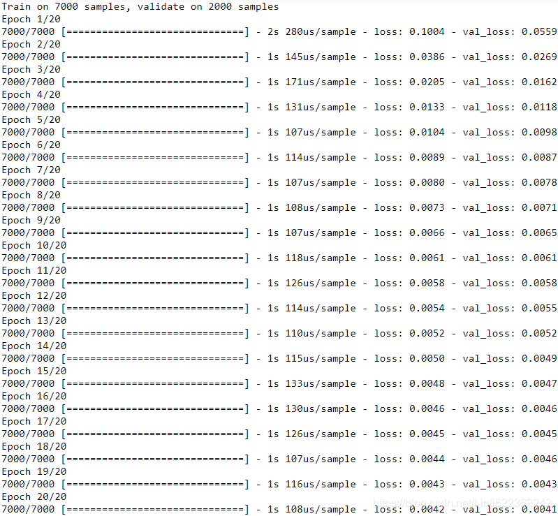

If we compile this model using the MSE loss and the default Adam optimizer, then fit it on the training set for 20 epochs and evaluate it on the validation set, we get an MSE of about 0.004. That’s much better than the naive approach()!

model.evaluate( X_valid, y_valid )

the validation error is computed at the end of each epoch, while the training error is computed using a running mean during each epoch. So the training curve should be shifted by half an epoch to the left. 10_Introduction to Artificial Neural Networks w Keras_3_FashionMNIST_pydot_sparse_shift(0.)_plt_imgs_learing curve : https://blog.csdn.net/Linli522362242/article/details/106562190

import matplotlib as mpl

def plot_learning_curves(loss, val_loss):
    # the validation error is computed at the end of each epoch,
    # while the training error is computed using a running mean during each epoch. 
    # So the training curve should be shifted by half an epoch to the left.
    plt.plot( np.arange( len(loss) )-0.5, loss, "b.-", label="Training loss" )
    plt.plot( np.arange( len(val_loss) ), val_loss, "r.-", label="Validation loss" )
    
    plt.axis([1, 20, # epoch is from 1 to 20
              0, 0.05])
    # integer : bool, default: False
    # If True, ticks will take only integer values, provided at least min_n_ticks integers 
    # are found within the view limits.
    # ranslate.google.com/?sl=auto&tl=zh-CN&op=translate
    plt.gca().xaxis.set_major_locator( mpl.ticker.MaxNLocator(integer=True) )
    plt.legend( fontsize=14 )
    plt.xlabel("Epochs")
    plt.ylabel("Loss")
    plt.grid(True)

plot_learning_curves( history.history["loss"], history.history["val_loss"] )

plt.show()

<==mpl.ticker.MaxNLocator(integer=True)<==
For demostration, let's move the above curves to right by both plus 1 #(len(train loss-0.5+1)=len(loss)+0.5 and len(val_loss)+1):

import matplotlib as mpl

def plot_learning_curves(loss, val_loss): # both loss and val_loss are a list
    # the validation error is computed at the end of each epoch,
    # while the training error is computed using a running mean during each epoch. 
    # So the training curve should be shifted by half an epoch to the left.
    plt.plot( np.arange( len(loss) )+0.5, loss, "b.-", label="Training loss" )
    plt.plot( np.arange( len(val_loss) )+1, val_loss, "r.-", label="Validation loss" )
    
    plt.axis([0, 20, 0, 0.05])
    plt.gca().xaxis.set_major_locator( mpl.ticker.MaxNLocator(integer=True) )
    plt.legend( fontsize=14 )
    plt.xlabel("Epochs")
    plt.ylabel("Loss")
    plt.grid(True)

plot_learning_curves( history.history["loss"], history.history["val_loss"] )

plt.show()

 # prediction on all data in X_valid but only just focus on [50]
y_pred = model.predict( X_valid )
# first 0: first series, 
# second 0: the value is saved in third dimension(1 for univariate time series)
# X_valid.shape = (2000, 50, 1), 2000 series, 50 time steps, 1 for univariate
plot_series( X_valid[0, :, 0], y_valid[0,0], y_pred[0,0] )

Implementing a Simple RNN

Let’s see if we can beat that with a simple RNN:
######################################
Using the TensorFlow Keras API, a recurrent layer can be defined via SimpleRNN, which is similar to the output-to-output recurrence.
https://blog.csdn.net/Linli522362242/article/details/113846940


# manually computing the output:
out_to_out = []
for t in range( len(x_seq) ):
    xt = tf.reshape( x_seq[t], (1,5) )
    print( "Time step {} =>".format(t) )
    print( '   Input           :', xt.numpy() )
    
    ht = tf.matmul(xt, w_xh) + b_h         ###########
    print('   Hidden          :', ht.numpy())
    
    if t>0:
        prev_output = out_to_out[t-1]
    else:
        prev_output = tf.zeros(shape=(ht.shape))
    
    ot = ht + tf.matmul(prev_output, w_oo) ###########
    ot = tf.math.tanh(ot) # since the activation in SimpleRNN is 'tanh'
    out_to_out.append(ot)
    
    print('   Output (manual) :', ot.numpy())
    print('   SimpleRNN output: '.format(t), 
          output[0][t].numpy())
    print()

######################################
since adam : default lr=0.001, let's increase it to 0.005

the behavior of a recurrent layer with respect to returning a sequence as output or simply using the last output can be specified by setting the argument return_sequences to True or False, respectively.

np.random.seed(42)
tf.random.set_seed(42)

model = keras.models.Sequential([
    keras.layers.SimpleRNN( 1, input_shape=[None,1] ) # default: use_bias=True, return_sequences=False
])

optimizer=keras.optimizers.Adam(lr=0.005) # adam : default lr=0.001

model.compile( loss="mse", optimizer=optimizer )
history = model.fit( X_train, y_train, epochs=20,
                     validation_data=(X_valid, y_valid) )

That’s really the simplest RNN you can build. It just contains a single layer, with a single neuron, as we saw in Figure 15-1. We do not need to specify the length of the input sequences (input_shape=[None,1]unlike in the previous model), since a recurrent neural network can process any number of time steps (this is why we set the first input dimension to None). By default, the SimpleRNN layer uses the hyperbolic tangent activation function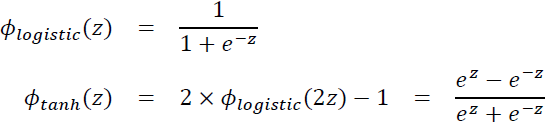. It works exactly as we saw earlier: the initial state is set to 0, and it is passed to a single recurrent neuron(for output), along with the value of the first time step, . The neuron computes a weighted sum of these values (### ht=tf.matmul(xt, w_xh) + b_h ; ot = ht + tf.matmul(prev_output, w_oo) ###)
and applies the hyperbolic tangent activation function to the result (### ot = tf.math.tanh(ot) ###),
and this gives the first output, (### out_to_out.append(ot) ###).
In a simple RNN, this output is also the new state (###prev_output = out_to_out[t-1]###).
This new state is passed to the same recurrent neuron along with the next input value, , and the process is repeated until the last time step. Then the layer just outputs the last value, . All of this is performed simultaneously for every time series.
#######################################
By default, recurrent layers in Keras only return the final output. To make them return one output per time step, you must set return_sequences=True, as we will see.
#######################################

If you compile, fit, and evaluate this model (just like earlier, we train for 20 epochs using Adam), you will find that its MSE reaches only 0.01, so it is better than the naive approach but it does not beat a simple linear model.### val_loss(here is "mse")=0.004145486235618591 ###
Note that for each neuron, a linear model has one parameter per input(### input features, here is 1 ###) and per time step, plus a bias term (in the simple linear model we used, that’s a total of 51=50+1 parameters). In contrast, for each recurrent neuron in a simple RNN, there is just one parameter per input(### input features, here is 1 : input_shape=[None,1]###) and per hidden state dimension
e.g. 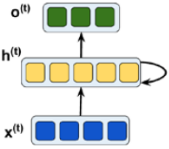h(t) dimension: 1x5
(in a simple RNN ###output-to-output recurrence###, that’s just the number of recurrent neurons in the layer ### keras.layers.SimpleRNN( 1,...) ### ), plus a bias term. In this simple RNN, that’s a total of just three parameters.(### The weight coefficients can be obtained during the training process, so they is no longer considered ###)

model.evaluate(X_valid, y_valid)

import matplotlib as mpl

def plot_learning_curves(loss, val_loss):
    # the validation error is computed at the end of each epoch,
    # while the training error is computed using a running mean during each epoch. 
    # So the training curve should be shifted by half an epoch to the left.
    plt.plot( np.arange( len(loss) )+0.5, loss, "b.-", label="Training loss" )
    plt.plot( np.arange( len(val_loss) )+1, val_loss, "r.-", label="Validation loss" )
    
    plt.axis([1, 20, 0, 0.05])###
    plt.gca().xaxis.set_major_locator( mpl.ticker.MaxNLocator(integer=False) )
    plt.legend( fontsize=14 )
    plt.xlabel("Epochs")
    plt.ylabel("Loss")
    plt.grid(True)

plot_learning_curves( history.history["loss"], history.history["val_loss"] )

plt.show()

 # prediction on all data in X_valid but only just focus on [50]
y_pred = model.predict( X_valid )
# first 0: first series, 
# second 0: the value is saved in third dimension(1 for univariate time series)
# X_valid.shape = (2000, 50, 1), 2000 series, 50 time steps, 1 for univariate
plot_series( X_valid[0, :, 0], y_valid[0,0], y_pred[0,0] )

#######################################

Trend and Seasonality

There are many other models to forecast time series, such as weighted moving average models (https://blog.csdn.net/Linli522362242/article/details/102314389) or autoregressive integrated moving average (ARIMA) models. Some of them require you to first remove the trend and seasonality. For example,

if you are studying the number of active users on your website, and it is growing by 10% every month, you would have to remove this trend from the time series. Once the model is trained and starts making predictions, you would have to add the trend back to get the final predictions.
Similarly, if you are trying to predict the amount of sunscreen lotion sold every month, you will probably observe strong seasonality: since it sells well every summer, a similar pattern will be repeated every year. You would have to remove this seasonality from the time series, for example by computing the difference between the value at each time step and the value one year earlier (this technique is called differencing). Again, after the model is trained and makes predictions, you would have to add the seasonal pattern back to get the final predictions.

When using RNNs, it is generally not necessary to do all this, but it may improve performance in some cases, since the model will not have to learn the trend or the seasonality.
#######################################

Apparently our simple RNN was too simple to get good performance. So let’s try to add more recurrent layers!

Deep RNNs

It is quite common to stack multiple layers of cells, as shown in Figure 15-7. This gives you a deep RNN.
Figure 15-7. Deep RNN (left) unrolled through time (right)

Implementing a deep RNN with tf.keras is quite simple: just stack recurrent layers. In this example, we use three SimpleRNN layers (but we could add any other type of recurrent layer, such as an LSTM layer or a GRU layer, which we will discuss shortly):

# the last layer use a SimpleRNN layer

np.random.seed(42)
tf.random.set_seed(42)

model = keras.models.Sequential([
    keras.layers.SimpleRNN( 20, return_sequences=True, input_shape=[None,1] ),
    keras.layers.SimpleRNN( 20, return_sequences=True),
    keras.layers.SimpleRNN(1)
])

model.compile( loss="mse", optimizer="adam" )
history = model.fit( X_train, y_train, epochs=20,
                     validation_data=(X_valid, y_valid) 
                   )

### the last layer use a SimpleRNN layer

##################

Make sure to set return_sequences=True for all recurrent layers (except the last one, if you only care about the last output). If you don’t, they will output a 2D array (containing only the output of the last time step with features,
########
e.g.• is an matrix containing the layer’s outputs at time step t for each instance in the mini-batch (m is the number of instances in the mini-batch and is the number output of neurons).
########
) instead of a 3D array (containing outputs for all time steps), and the next recurrent layer will complain that you are not feeding it sequences in the expected 3D format.
##################

If you compile, fit, and evaluate this model, you will find that it reaches an MSE of 0.003. We finally managed to beat the linear model ### val_loss(here is "mse")=0.004145486235618591 ### !

model.evaluate( X_valid, y_valid )

plot_learning_curves( history.history["loss"], history.history["val_loss"])

plt.show()

y_pred = model.predict(X_valid)
plot_series( X_valid[0, :, 0], y_valid[0,0], y_pred[0,0] )

plt.show()

Note that the last layer ### keras.layers.SimpleRNN(1) ### is not ideal: it must have a single unit because we want to forecast a univariate time series(there is a single value per time step), and this means we must have a single output value per time step. However, having a single unit means that the hidden state is just a single number. That’s really not much, and it’s probably not that useful; presumably, the RNN will mostly use the hidden states of the other recurrent layers to carry over all the information it needs from time step to time step, and it will not use the final layer’s hidden state very much. Moreover, since a SimpleRNN layer uses the tanh activation function by default, the predicted values must lie within the range –1 to 1. But what if you want to use another activation function? For both these reasons, it might be preferable to replace the output layer with a Dense layer: it would run slightly faster, the accuracy would be roughly the same, and it would allow us to choose any output activation function we want. If you make this change, also make sure to remove return_sequences=True from the second (now last) recurrent layer:

# the last layer use a Dense layer

np.random.seed(42)
tf.random.set_seed(42)

model = keras.models.Sequential([
    keras.layers.SimpleRNN(20, return_sequences=True, input_shape=[None,1]),
    keras.layers.SimpleRNN(20), ########### many to one OR sequence-to-vector(vector: features)
    keras.layers.Dense(1) # activation=None
])

model.compile( loss="mse", optimizer="adam" )
history = model.fit( X_train, y_train, epochs=20,
                     validation_data=(X_valid, y_valid)
                   )

If you train this model, you will see that it converges faster and performs just as well. Plus, you could change the output activation function if you wanted.

model.evaluate(X_valid, y_valid)

plot_learning_curves( history.history["loss"], history.history["val_loss"] )

plt.show()

y_pred = model.predict( X_valid )
plot_series( X_valid[0, :, 0], y_valid[0,0], y_pred[0,0] )

plt.show()

Forecasting Several Time Steps Ahead

So far we have only predicted the value at the next time step, but we could just as easily have predicted the value several steps ahead by changing the targets appropriately (e.g., to predict 10 steps ahead, just change the targets to be the value 10 steps ahead instead of 1 step ahead). But what if we want to predict the next 10 values?

# RNN predicts next 10 values 1 by 1

The first option is to use the model we already trained, make it predict the next value, then add that value to the inputs (acting as if this predicted value had actually occurred), and use the model again to predict the following value, and so on, as in the following code:

import numpy as np

def generate_time_series(batch_size, n_steps):
    freq1, freq2, offsets1, offsets2 = np.random.rand(4, batch_size, 1)
    # print(freq1.shape) # (batches,1)
    time = np.linspace(0,1, n_steps) 
    # print(time.shape)  # (n_steps,)
    
    # https://numpy.org/doc/stable/user/basics.broadcasting.html
    # time-offsets1 shape: (n_steps,)-(batches,1) 
    # the axes operation is from right to left : 
    #                         time.shape(n_steps,)         - freq1.shape(batches,1)
    #                      ==>time.shape(,n_steps)         - freq1.shape(batches,1)
    # broadcast operation  ==>time.shape(batches, n_steps) along row(batches)
    #                         - offsets1.shape(batches,n_steps) along column(,n_steps)
    #                       result.shape(batches,n_steps)
    series = 0.5*np.sin( (time-offsets1)*(freq1*10 + 10) )  # wave 1 in the 1st row
    #print(series.shape) # (batches, n_steps+1)
    series += 0.2*np.sin( (time-offsets2)*(freq2*20 + 20) ) # +wave 2 in the 2nd row
    # print(series.shape) # (batches, n_steps)
    series += 0.1*(np.random.rand(batch_size, n_steps)-0.5) # +noise in the 3rd row
    # print(series.shape) # (batches, n_steps)
    
    return series[..., np.newaxis].astype( np.float32 )

np.random.seed(43) # not 42, as it would give the first series in the train set

##################################################
   # def generate_time_series(batch_size, n_steps)
series = generate_time_series(1, n_steps + 10) # n_steps=50
X_new, Y_new = series[:, :n_steps], series[:, n_steps:] #  the errors might accumulate

X = X_new
# X.shape # (1, 50, 1)

for step_ahead in range(10): 
    # Forecasting 10 steps ahead, 1 step at a time; then expand dimension to
    # [batch size,time steps,dimensions]
    y_pred_one = model.predict( X[:, step_ahead:] )[:, np.newaxis, :] ############

    X = np.concatenate([X, y_pred_one], axis=1)
    
Y_pred = X[:, n_steps:]
Y_pred.shape

def plot_multiple_forecasts( X,Y,Y_pred):
    n_steps = X.shape[1]
    ahead = Y.shape[1]
    
    plot_series(X[0, :, 0]) # first series in X
    plt.plot( np.arange(n_steps, n_steps+ahead), Y[0, :, 0],
              "yo-", label="Actual" )
    plt.plot( np.arange(n_steps, n_steps+ahead), Y_pred[0, :, 0],
              "bx-", label="Forecast", markersize=10 )
    
    plt.axis([0, n_steps+ahead, -1, 1])
    plt.legend( fontsize=14 )
    
plot_multiple_forecasts( X_new, Y_new, Y_pred )
plt.show()

Figure 15-8. Forecasting 10 steps ahead, 1 step at a time

As you might expect, the prediction for the next step will usually be more accurate than the predictions for later time steps( vs ), since the errors might accumulate (as you can see in Figure 15-8). If you evaluate this approach on the validation set, you will find an MSE of about 0.029. This is much higher than the previous models, but it’s also a much harder task, so the comparison doesn’t mean much. It’s much more meaningful to compare this performance with naive predictions (just forecasting that the time series will remain constant for 10 time steps) or with a simple linear model. The naive approach is terrible (it gives an MSE of about 0.22), but the linear model gives an MSE of about 0.0188: it’s much better than using our RNN to forecast the future one step at a time, and also much faster to train and run. Still, if you only want to forecast a few time steps ahead, on more complex tasks, this approach may work well.

# OR # np.mean( keras.metrics.mean_squared_error( Y_new, Y_pred ))
np.mean( keras.losses.mean_squared_error( Y_new, Y_pred ))

^^^^^^^^^^^^^^^^^^^^^^^^^^^^^^^^^^^^^^^^^^^^^

np.random.seed(43) # not 42, as it would give the first series in the train set

   # def generate_time_series(batch_size, n_steps)
series = generate_time_series(1, n_steps + 10) # n_steps=50
X_new, Y_new = series[:, :n_steps], series[:, n_steps:]

X = X_new
# X.shape # (1, 50, 1)

for step_ahead in range(10): 
    #use next 10 time_steps for predition then expand dimension to[batch size,time steps,dimensionality]
    y_pred_one = model.predict( X )[:, np.newaxis, :]############
    X = np.concatenate([X, y_pred_one], axis=1)
    
Y_pred = X[:, n_steps:]

def plot_multiple_forecasts( X,Y,Y_pred):
    n_steps = X.shape[1]
    ahead = Y.shape[1]
    
    plot_series(X[0, :, 0]) # first series in X
    plt.plot( np.arange(n_steps, n_steps+ahead), Y[0, :, 0],
              "yo-", label="Actual" )
    plt.plot( np.arange(n_steps, n_steps+ahead), Y_pred[0, :, 0],
              "bx-", label="Forecast", markersize=10 )
    
    plt.axis([0, n_steps+ahead, -1, 1])
    plt.legend( fontsize=14 )
    
plot_multiple_forecasts( X_new, Y_new, Y_pred )
plt.show()

From the graphic point of view, the forecast trend curve made using the entire data set (including the original data + gradually added data) and the fixed-length data set (the latter part of the original data + the gradually added data) looks the same, but The loss function (mse) is different (since the errors accumulated are different)

np.mean( keras.losses.mean_squared_error( Y_new, Y_pred ))

The reason is the timeliness of the data (the newer the data, the more accurate the forecast (since the errors accumulated are different))

#################

# np.random.seed(42)
# tf.random.set_seed(42)

# model = keras.models.Sequential([
#     keras.layers.SimpleRNN(20, return_sequences=True, input_shape=[None,1]),
#     keras.layers.SimpleRNN(20),
#     keras.layers.Dense(1)
# ])

# model.compile( loss="mse", optimizer="adam" )
# history = model.fit( X_train, y_train, epochs=20,
#                      validation_data=(X_valid, y_valid)
#                    )

let's predict the next 10 values one by one:
# the fixed-length data set (the latter part of the original data + the gradually added data((predictions)))

np.random.seed(42)

n_steps = 50
series = generate_time_series(10000, n_steps+10) # n_steps=50
                        # (7000, 50, 1)          # (7000, 10)
X_train, Y_train = series[:7000, :n_steps], series[:7000, -10:, 0]
X_valid, Y_valid = series[7000:9000, :n_steps], series[7000:9000, -10:, 0]
X_test, Y_test = series[9000:, :n_steps], series[9000:, -10:, 0]
# X_train.shape # (7000, 50, 1)

X = X_valid # (2000, 50, 1)

for step_ahead in range(10):
    # Forecasting 10 steps ahead, 1 step at a time; then expand dimension to
    # [batch size,time steps,dimensions]
    y_pred_one = model.predict(X[:, step_ahead:])[:, np.newaxis, :] ###################
    X = np.concatenate( [X, y_pred_one], axis=1 )

Y_pred = X[:, n_steps:, 0] 
# Y_pred.shape  # (2000, 10)

np.mean(keras.metrics.mean_squared_error(Y_valid, Y_pred))

The reason is the timeliness of the data (the newer the data, the more accurate the forecast (since the errors accumulated are different))
VVVVVVVVVVVVVVVVVVVVVVVVVVVVVVVV

np.random.seed(42)

n_steps = 50
series = generate_time_series(10000, n_steps+10) # n_steps=50
                        # (7000, 50, 1)          # (7000, 10)
X_train, Y_train = series[:7000, :n_steps], series[:7000, -10:, 0]
X_valid, Y_valid = series[7000:9000, :n_steps], series[7000:9000, -10:, 0]
X_test, Y_test = series[9000:, :n_steps], series[9000:, -10:, 0]
X_train.shape

Now let's predict the next 10 values one by one:
### the original data + gradually added data(predictions)

X = X_valid # (2000, 50, 1)

for step_ahead in range(10):
    # Forecasting 10 steps ahead, 1 step at a time; then expand dimension to
    # [batch size,time steps,dimensions]
    y_pred_one = model.predict(X)[:, np.newaxis, :]
    X = np.concatenate( [X, y_pred_one], axis=1 )

Y_pred = X[:, n_steps:, 0] 
Y_pred.shape # (2000, 10)

As you might expect, the prediction for the next step will usually be more accurate than the predictions for later time steps( vs ), since the errors might accumulate (as you can see in Figure 15-8). If you evaluate this approach on the validation set, you will find an MSE of about 0.027. It’s much more meaningful to compare this performance with naive predictions (just forecasting that the time series will remain constant for 10 time steps) or with a simple linear model. The naive approach is terrible (it gives an MSE of about 0.22), but the linear model gives an MSE of about 0.0188: it’s much better than using our RNN to forecast the future one step at a time, and also much faster to train and run. Still, if you only want to forecast a few time steps ahead, on more complex tasks, this approach may work well.

np.mean(keras.metrics.mean_squared_error(Y_valid, Y_pred))

The reason is the timeliness of the data (the newer the data, the more accurate the forecast)

Let's compare this performance with some baselines: naive predictions and a simple linear model:

# naive predictions

# Y_valid.shape # (2000, 10)
Y_naive_pred = Y_valid[:, -1:] # (2000, 1)
# (2000, 1)
                                         # exists a broadcasting operation
np.mean(keras.metrics.mean_squared_error(Y_valid, Y_naive_pred))

# the linear model

np.random.seed(42)
tf.random.set_seed(42)

model = keras.models.Sequential([
    keras.layers.Flatten(input_shape=[50,1]),
    keras.layers.Dense(10)
])

model.compile( loss="mse", optimizer="adam" )
history = model.fit(X_train, Y_train, epochs=20,
                    validation_data=(X_valid, Y_valid)
                   )

The second option is to train an RNN to predict all 10 next values at once. We can still use a sequence-to-vector model(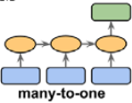), but it will output 10 values instead of 1. However, we first need to change the targets to be vectors containing the next 10 values:

# np.random.seed(42)

# n_steps = 50
# series = generate_time_series(10000, n_steps+10) # n_steps=50
                        # (7000, 50, 1)          # (7000, 10)
# X_train, Y_train = series[:7000, :n_steps], series[:7000, -10:, 0]
# X_valid, Y_valid = series[7000:9000, :n_steps], series[7000:9000, -10:, 0]
# X_test, Y_test = series[9000:, :n_steps], series[9000:, -10:, 0]

# RNN predicts all 10 next values(target batch_size x 10) at once and only at the very last time step:

### keras.layers.SimpleRNN(20, return_sequences=False) ###
Now we just need the output layer to have 10 units instead of 1 (### keras.layers.Dense(10) ###):

np.random.seed(42)
tf.random.set_seed(42)

model = keras.models.Sequential([
    keras.layers.SimpleRNN(20, return_sequences=True, input_shape=[None,1]),
    keras.layers.SimpleRNN(20), # many-to-1 : sequence-to-vector(vector: features)
    keras.layers.Dense(10)      # sequence is a time series(with "many" time steps)
])                              # 1: last 1 time step with multiple features, here just one feature

model.compile( loss="mse", optimizer="adam")
history = model.fit(X_train, Y_train, epochs=20,
                    validation_data=(X_valid, Y_valid))

After training this model, you can predict the next 10 values at once very easily:

np.random.seed(43)

series = generate_time_series(1, 50+10) # 1 instance with 50+10 time steps
X_new, Y_new = series[:, :50, :], series[:, -10:, :]
Y_pred = model.predict(X_new)[..., np.newaxis] # prediction then expand dimension to [batch_size, steps, features]
Y_pred

plot_multiple_forecasts(X_new, Y_new, Y_pred)

plt.show()

This model works nicely: the MSE for the next 10 time steps is about 0.008(). That’s much better than the linear model(). But we can still do better: indeed, instead of training the model to forecast the next 10 values only at the very last time step, we can train it to forecast the next 10 values at each and every time step.

forecast the next 10 values at each and every time step

In other words, we can turn this sequence-to-vector RNN into a sequence-to-sequence RNN. The advantage of this technique is that

the loss will contain a term for the output of the RNN at each and every time step, not just the output at the last time step.
This means there will be many more error gradients flowing through the model, and they won’t have to flow only through time; they will also flow from the output of each time step.
This will both stabilize and speed up training.

Now let's create an RNN that predicts the next 10 steps at each time step. That is, instead of just forecasting time steps 50 to 59 based on time steps 0 to 49, it will forecast time steps 1 to 10 at time step 0, then time steps 2 to 11 at time step 1, and so on, and finally it will forecast time steps 50 to 59 at the last time step. (Notice that the model is causal: when it makes predictions at any time step, it can only see past time steps). So each target must be a sequence of the same length as the input sequence, containing a 10-dimensional vector at each step.

Let’s prepare these target sequences:

np.random.seed(42)

n_steps = 50
series = generate_time_series(10000, n_steps+10) # 10000x60x1
X_train = series[:7000, :n_steps] # 7000x50x1
X_valid = series[7000:9000, :n_steps]
X_test = series[9000:, :n_steps]

Y = np.empty( (10000, n_steps, 10) ) #  # 10000x50x10
for step_ahead in range(1, 10+1): # Y :0     1     2          9     #[,rows=n_steps, column_index] 
    # Y[..., 0~9]                    # 1~50, 2~51, 3~52, ..., 10~59     # row range at each loop 
    Y[..., step_ahead-1] = series[..., step_ahead:step_ahead+n_steps, 0]# get 50 data at each loop

Y_train = Y[:7000]
Y_valid = Y[7000:9000]
Y_test = Y[9000:]

X_train.shape, Y_train.shape

#########################

If a sequence : Deep ... Learni...

first time step in X: D

--> (Horizontal) Column
2nd time step in X: e

--> (Horizontal) Column

series[0, 0:1+n_steps, 0] # n steps=50

step_ahead=1

series[0, 1:1+n_steps, 0] # n steps=50

step_ahead=1

Y[0,...,1-1]

step_ahead=2

Y[0,...,2-1]

Y[0,0] # first time step

# X_train: [batch_size, steps, features]
X_train[0,0] # the first time step in the first instance

Y_train[0,0] # the first time step in the first target

# X_train: [batch_size, steps, features]
X_train[0,1] # the 2nd time step in the first instance

Y_train[0,1] # the 2nd time step in the first target

#########################
####################################################

It may be surprising that the targets will contain values that appear in the inputs (there is a lot of overlap between X_train and Y_train). Isn’t that cheating? Fortunately, not at all: at each time step, the model only knows about past time steps, so it cannot look ahead. It is said to be a causal model.
####################################################TimeDistributed layer

To turn the model into a sequence-to-sequence model, we must set return_sequences=True in all recurrent layers (even the last one), and we must apply the output Dense layer at every time step. Keras offers a
TimeDistributed layer for this very purpose: it wraps any layer (e.g., a Dense layer) and applies it at every time step of its input sequence. It does this efficiently, by reshaping the inputs so that each time step is treated as a separate instance

(i.e., it reshapes the inputs from [batch size, time steps, input dimensions] to [batch size × time steps, input dimensions]; in this example, the number of input dimensions is 20 because the previous SimpleRNN layer has 20 units),
then it runs the Dense layer, and
finally it reshapes the outputs back to sequences (i.e., it reshapes the outputs from [batch size × time steps, output dimensions] to [batch size, time steps, output dimensions]; in this example the number of output dimensions is 10, since the Dense layer has 10 units).### Note that a TimeDistributed(Dense(n)) layer is equivalent to a Conv1D(n, filter_size=1) layer. ###

Here is the updated model:

np.random.seed(42)
tf.random.set_seed(42)

model = keras.models.Sequential([
    keras.layers.SimpleRNN( 20, return_sequences=True, input_shape=[None, 1] ),
    keras.layers.SimpleRNN( 20, return_sequences=True ),#forecast the next 10 values at each and every time step
    keras.layers.TimeDistributed( keras.layers.Dense(10) )
])

def last_time_step_mse( Y_true, Y_pred):  # ":" represents all instances, "-1" is last time step
    return keras.metrics.mean_squared_error( Y_true[:, -1], Y_pred[:, -1] )

model.compile( loss="mse", optimizer=keras.optimizers.Adam( lr=0.01 ),
               metrics = [last_time_step_mse] )

history = model.fit( X_train, Y_train, epochs=20,
                     validation_data=(X_valid, Y_valid) )

The Dense layer actually supports sequences as inputs (and even higher-dimensional inputs): it handles them just like TimeDistributed(Dense(…)), meaning it is applied to the last input dimension only (independently across all time steps). Thus, we could replace the last layer with just Dense(10). For the sake of clarity, however, we will keep using TimeDistributed(Dense(10)) because it makes it clear that the Dense layer is applied independently at each time step and that the model will output a sequence[batch size, time steps, output dimensions], not just a single vector.

All outputs are needed during training, but only the output at the last time step is useful for predictions and for evaluation. So although we will rely on the MSE over all the outputs for training, we will use a custom metric for evaluation, to only compute the MSE over the output at the last time step.

We get a validation MSE of about 0.006, which is 25%(1-0.006/0.008=1-0.75=0.25) better than the previous model. You can combine this approach with the first one: just predict the next 10 values using this RNN, then concatenate these values to the input time series and use the model again to predict the next 10 values, and repeat the process as many times as needed. With this approach, you can generate arbitrarily long sequences. It may not be very accurate for long-term predictions, but it may be just fine if your goal is to generate original music or text, as we will see in Chapter 16.

np.random.seed(43)

series = generate_time_series(1, 50+10) # create 1 instance with 50+10 time steps
X_new, Y_new = series[:, :50, :], series[:, 50:, :] # first 50 time steps as X_new for prediction,
                                                    # the last 10 time steps as actual Y
# ":" represents all instances, "-1" is last time step
# model.predict(X_new)[:, -1] is a 1D list then expand its dimention to 2D
Y_pred = model.predict(X_new)[:, -1][..., np.newaxis]
Y_pred

plot_multiple_forecasts(X_new, Y_new, Y_pred)
plt.show()

Simple RNNs can be quite good at forecasting time series or handling other kinds of sequences, but they do not perform as well on long time series or sequences. Let’s discuss why and see what we can do about it.

Handling Long Sequences

To train an RNN on long sequences, we must run it over many time steps, making the unrolled RNN a very deep network. Just like any deep neural network it may suffer from the unstable gradients problem( This is when the gradients grow smaller and smaller, or larger and larger), discussed in Chapter 11 : https://blog.csdn.net/Linli522362242/article/details/106935910: it may take forever to train, or training may be unstable. Moreover, when an RNN processes a long sequence, it will gradually forget the first inputs in the sequence. Let’s look at both these problems, starting with the unstable gradients problem.

Fighting the Unstable Gradients Problem

Many of the tricks we used in deep nets to alleviate减轻 the unstable gradients problem can also be used for RNNs: good parameter initialization, faster optimizers, dropout, and so on. However, nonsaturating activation functions (e.g., ReLU) may not help as much here; in fact, they may actually lead the RNN to be even more unstable during training. Why? Well, suppose Gradient Descent updates the weights in a way that increases the outputs slightly at the first time step. Because the same weights are used at every time step, the outputs at the second time step may also be slightly increased, and those at the third, and so on until the outputs explode—and a nonsaturating activation function does not prevent that. You can reduce this risk by using a smaller learning rate, but you can also simply use a saturating activation function like the hyperbolic tangent (this explains why it is the default). In much the same way, the gradients themselves can explode. If you notice that training is unstable, you may want to monitor the size of the gradients (e.g., using TensorBoard) and perhaps use Gradient Clippinghttps://blog.csdn.net/Linli522362242/article/details/106935910.

Moreover, Batch Normalization(https://blog.csdn.net/Linli522362242/article/details/106935910) cannot be used as efficiently with RNNs as with deep feedforward nets. In fact, you cannot use it between time steps, only between recurrent layers. To be more precise, it is technically possible to add a BN layer to a memory cell (as we will see shortly) so that it will be applied at each time step (both on the inputs for that time step and on the hidden state from the previous step). However, the same BN layer will be used at each time step, with the same parameters, regardless of the actual scale and offset of the inputs and hidden state. In practice, this does not yield good results, as was demonstrated by César Laurent et al. in a 2015 paper:3 the authors found that BN was slightly beneficial only when it was applied to the inputs, not to the hidden states. In other words, it was slightly better than nothing when applied between recurrent layers (i.e., vertically in Figure 15-7), but not within recurrent layers (i.e., horizontally). In Keras this can be done simply by adding a Batch Normalization layer before each recurrent layer, but don’t expect too much from it.
###########
It is quite common to stack multiple layers of cells, as shown in Figure 15-7. This gives you a deep RNN.
Figure 15-7. Deep RNN (left) unrolled through time (right)
###########

np.random.seed(42)
tf.random.set_seed(42)

model = keras.models.Sequential([
    keras.layers.SimpleRNN(20, return_sequences=True, input_shape=[None,1] ),
    
    keras.layers.BatchNormalization(), # was applied to the inputs
    keras.layers.SimpleRNN(20, return_sequences=True),
    
    keras.layers.BatchNormalization(),
    keras.layers.TimeDistributed( keras.layers.Dense(10) ) # output: 10 next 10 time steps' value
])

model.compile( loss="mse", optimizer="adam", metrics=[last_time_step_mse] )
history = model.fit( X_train, Y_train, epochs=20,
                     validation_data=(X_valid, Y_valid) 
                   )

Another form of normalization often works better with RNNs: Layer Normalization. This idea was introduced by Jimmy Lei Ba et al. in a 2016 paper(Jimmy Lei Ba et al., “Layer Normalization,” arXiv preprint arXiv:1607.06450 (2016).): it is very similar to Batch Normalization, but instead of normalizing across the batch dimension, it normalizes across the features dimension. One advantage is that it can compute the required statistics on the fly, at each time step, independently for each instance. This also means that it behaves the same way during training and testing
(### as opposed to BN,https://blog.csdn.net/Linli522362242/article/details/106935910

Batch Normalization 是对这批所有样本的各个(independent)特征维度分别做归一化（6次）， Layer Normalization 是对这单个样本的所有(across)特征维度做归一化（3次）
将输入的图像shape记为[N, C, H, W]，这几个方法主要的区别就是在
N_y 表示样本轴， C_x表示通道轴， F_z是每个通道的特征数量（here is 2 since [H,W]）。

BN是先一个通道（在多层神经元中就是某一层的纬度或者神经元的节点数目），接着在同一批所有样本的的一个(independent)特征，一个(independent)特征的做归一化, （或者说在batch上，对NHW做归一化），然后在下一个通道（对小batchsize效果不好）
LN则是先一个样本，一个通道的所有(across)特征维度，一个通道的所有(across)特征维度做归一化。（或者说对CHW做归一化）,然后下一个样本 https://blog.csdn.net/Linli522362242/article/details/107596098
Equation 11-3. Batch Normalization algorithm
https://blog.csdn.net/Linli522362242/article/details/106935910
Durint training: the Batch Normalization algorithm needs to estimate each input’s mean and standard deviation. It does so by evaluating the mean and standard deviation of the input over the current mini-batch. So during training, BN standardizes its inputs, then rescales and offsets them.
at test time:
One solution could be to wait until the end of training, then run the whole training set through the neural network and compute the mean and standard deviation of each input of the BN layer. These “final” input means and standard deviations could then be used instead of the batch input means and standard deviations when making predictions.

However, most implementations of Batch Normalization estimate these final statistics during training by using a moving average of the layer’s input means and standard deviations. This is what Keras does automatically when you use the BatchNormalization layer. To sum up, four parameter vectors are learned in each batch-normalized layer: γ (the output scale vector) and
β (the output offset vector) are learned through regular backpropagation, and
μ (the final input mean vector) and
σ (the final input standard deviation vector) are estimated using an exponential moving average. Note that μ and σ are estimated during training, but they are used only after training (to replace the batch input means and standard deviations in Equation 11-3).

### ), and it does not need to use exponential moving averages to estimate the feature statistics across all instances in the training set. Like BN, Layer Normalization learns a scale and an offset parameter for each input. In an RNN, it is typically used right after the linear combination of the inputs and the hidden states.

Let’s use tf.keras to implement Layer Normalization within a simple memory cell. For this, we need to define a custom memory cell. It is just like a regular layer, except its

call() method takes two arguments: the inputs at the current time step and the hidden states from the previous time step. Note that the states argument is a list containing one or more tensors.
In the case of a simple RNN cell it contains a single tensor equal to the outputs of the previous time step, but other cells may have multiple state tensors (e.g., an LSTMCell has a long-term state and a short-term state, as we will see shortly). A cell must also have a state_size attribute and an output_size attribute. In a simple RNN, both are simply equal to the number of units.

The following code implements a custom memory cell which will behave like a SimpleRNNCell, except it will also apply Layer Normalization at each time step:

from tensorflow.keras.layers import LayerNormalization

class LNSimpleRNNCell( keras.layers.Layer ):
    def __init__( self, units, activation="tanh", **kwargs ):
        super().__init__( **kwargs )
        self.state_size = units
        self.output_size = units
        self.simple_rnn_cell = keras.layers.SimpleRNNCell( units, # Positive integer, dimensionality of the output space.
                                                           activation=None 
                                                         )# processes one step within the whole time sequence input
        # tf.keras.layers.LayerNormalization
        #                Normalize the activations of the previous layer for "each given example" in a batch "independently",
        #                rather than "across a batch" like Batch Normalization.
        #                i.e. applies a transformation that maintains the mean activation "within each example" close to 0 
        #                     and the activation standard deviation close to 1.
        # within each example : across all feature dimensions do normalization
        self.layers_norm = LayerNormalization()
        self.activation = keras.activations.get(activation)
        
    def get_initial_state( self, inputs=None, batch_size=None, dtype=None ):
        if inputs is not None:
            batch_size = tf.shape(inputs)[0]
            dtype = inputs.dtype
        return [tf.zeros([batch_size, self.state_size])]
    
    def call( self, inputs, states):
        # keras.layers.SimpleRNNCell
        #                       processes one step within the whole time sequence input, 
        #                       whereas tf.keras.layer.SimpleRNN processes the whole sequence.
        #                inputs: A 2D tensor, with shape of [batch, feature].
        #                states: A 2D tensor with shape of [batch, units], which is the state from the previous time step. 
        #                       For timestep 0, the initial state provided by user will be feed to cell.
        #                       the states argument is a list containing one or more tensors.
        # simple RNN cell, which computes a linear combination of the current inputs and the previous hidden states, 
        # and it returns the result twice (indeed, in a SimpleRNNCell, the outputs are just equal to the hidden states
        # states: in other words, new_states[0] is equal to outputs
        outputs, new_states = self.simple_rnn_cell(inputs, states)
        # perform Layer Normalization before the activation function
        norm_outputs = self.activation( self.layers_norm(outputs) )
        return norm_outputs, [norm_outputs] # once as the outputs, and once as the new hidden states

The code is quite straightforward (It would have been simpler to inherit from SimpleRNNCell instead so that we wouldn’t have to create an internal SimpleRNNCell or handle the state_size and output_size attributes, but the goal here was to show how to create a custom cell from scratch.). Our LNSimpleRNNCell class inherits from the keras.layers.Layer class, just like any custom layer.

The constructor takes the number of units and the desired activation function, and
it sets the state_size and output_size attributes, then
creates a SimpleRNNCell with no activation function (because we want to perform Layer Normalization after the linear operation but before the activation function). Then
the constructor creates the LayerNormalization layer, and finally it fetches the desired activation function.
The call() method starts by applying
the simple RNN cell, which computes a linear combination of the current inputs and the previous hidden states, and it returns the result twice (indeed, in a SimpleRNNCell, the outputs are just equal to the hidden states: in other words, new_states[0] is equal to outputs, so we can safely ignore new_states in the rest of the call() method).
Next, the call() method applies Layer Normalization,
followed by the activation function.
Finally, it returns the outputs twice (once as the outputs, and once as the new hidden states).
To use this custom cell, all we need to do is create a keras.layers.RNN layer, passing it a cell instance:

np.random.seed(42)
tf.random.set_seed(42)

model = keras.models.Sequential([
    # simple_rnn_cell==>layers_norm==>activation==>simple_rnn_cell==>...
    keras.layers.RNN( LNSimpleRNNCell(20), return_sequences=True,
                      input_shape=[None,1]),                       # return_sequences=True
    keras.layers.RNN( LNSimpleRNNCell(20), return_sequences=True ),# forecast the next 10 values at each and every time step
    keras.layers.TimeDistributed( keras.layers.Dense(10) ) # output: next 10 time steps' value
])

def last_time_step_mse( Y_true, Y_pred):  # ":" represents all instances, "-1" is last time step
    return keras.metrics.mean_squared_error( Y_true[:, -1], Y_pred[:, -1] )

model.compile( loss="mse", optimizer="adam", metrics=[last_time_step_mse] )
history = model.fit( X_train, Y_train, epochs=20,
                     validation_data=(X_valid, Y_valid) 
                   )

Similarly, you could create a custom cell to apply dropout between each time step. But there’s a simpler way: all recurrent layers (except for keras.layers.RNN) and all cells provided by Keras have a dropout hyperparameter and a recurrent_dropout hyperparameter: the former defines the dropout rate to apply to the inputs (at each time step), and the latter defines the dropout rate for the hidden states (also at each time step). No need to create a custom cell to apply dropout at each time step in an RNN.

With these techniques, you can alleviate the unstable gradients problem and train an RNN much more efficiently. Now let’s look at how to deal with the short-term memory problem.

Creating a Custom RNN Class

X_train.shape

class MyRNN( keras.layers.Layer ):
    def __init__( self, cell, return_sequences=False, **kwargs):
        super().__init__(**kwargs)
        self.cell = cell                                           # <== LNSimpleRNNCell(20)
        self.return_sequences = return_sequences
        self.get_initial_state = getattr(
            self.cell, "get_initial_state",                        # <== LNSimpleRNNCell.get_initial_state
            self.fallback_initial_state # If the named attribute("get_initial_state") does not exist, default is returned if provided
        )
        
    def fallback_initial_state( self, inputs ):
        return [ tf.zeros([self.cell.state_size],                   # LNSimpleRNNCell.state_size=units
                           dtype=inputs.dtype) ]
    
    @tf.function
    def call( self, inputs ):
        states = self.get_initial_state(inputs)
        n_steps = tf.shape( inputs )[1] # 50 time steps
        if self.return_sequences:
            sequences = tf.TensorArray(inputs.dtype, size=n_steps)
            
        outputs = tf.zeros( shape=[n_steps, self.cell.output_size],  # LNSimpleRNNCell.output_size=units
                            dtype=inputs.dtype)
        for step in tf.range(n_steps):
            # similar to outputs, new_states = self.simple_rnn_cell(inputs, states)
            outputs, states = self.cell( inputs[:, step], states )
            if self.return_sequences:
                sequences = sequences.write(step, outputs) # sequences[step]=outputs
        if self.return_sequences:
            # https://blog.csdn.net/z2539329562/article/details/80639199
            return sequences.stack() # All the tensors in the TensorArray stacked into one tensor.
        else:
            return outputs

np.random.seed(42)
tf.random.set_seed(42)

model = keras.models.Sequential([
    MyRNN( LNSimpleRNNCell(20), return_sequences=True,
           input_shape=[None,1]),
    MyRNN( LNSimpleRNNCell(20), return_sequences=True),
    keras.layers.TimeDistributed( keras.layers.Dense(10) )
])

model.compile( loss="mse", optimizer="adam", metrics = [last_time_step_mse])
history = model.fit(X_train, Y_train, epochs=20,
                    validation_data=(X_valid, Y_valid))

Tackling the Short-Term Memory Problem

Due to the transformations that the data goes through when traversing an RNN, some information is lost at each time step. After a while, the RNN’s state contains virtually no trace of the first inputs. This can be a showstopper. Imagine Dory the fish(A character from the animated movies Finding Nemo and Finding Dory海底总动员 who has short-term memory loss.) trying to translate a long sentence; by the time she’s finished reading it, she has no clue how it started. To tackle this problem, various types of cells with long-term memory have been introduced. They have proven so successful that the basic cells are not used much anymore. Let’s first look at the most popular of these long-term memory cells: the LSTM cell.

LSTM cells

The Long Short-Term Memory (LSTM) cell was proposed in 1997(Sepp Hochreiter and Jürgen Schmidhuber, “Long Short-Term Memory,” Neural Computation 9, no. 8 (1997):1735–1780) by Sepp Hochreiter and Jürgen Schmidhuber and gradually improved over the years by several researchers, such as Alex Graves, Haşim Sak(Haşim Sak et al., “Long Short-Term Memory Based Recurrent Neural Network Architectures for Large Vocabulary Speech Recognition,” arXiv preprint arXiv:1402.1128 (2014).), and Wojciech Zaremba(Wojciech Zaremba et al., “Recurrent Neural Network Regularization,” arXiv preprint arXiv:1409.2329 (2014).). If you consider the LSTM cell as a black box, it can be used very much like a basic cell, except it will perform much better; training will converge faster, and it will detect long-term dependencies in the data. In Keras, you can simply use the LSTM layer instead of the SimpleRNN layer:

np.random.seed(42)
tf.random.set_seed(42)

model = keras.models.Sequential([
    keras.layers.LSTM(20, return_sequences=True, input_shape=[None, 1]),
    keras.layers.LSTM(20, return_sequences=True),
    keras.layers.TimeDistributed( keras.layers.Dense(10) )
])

model.compile( loss="mse", optimizer="adam", metrics=[last_time_step_mse] )
history = model.fit( X_train, Y_train, epochs=20,
                     validation_data=(X_valid, Y_valid) 
                   )

Alternatively, you could use the general-purpose keras.layers.RNN layer, giving it an LSTMCell as an argument:

model = keras.models.Sequential([
    keras.layers.RNN( keras.layers.LSTMCell(20), return_sequences=True,
                      input_shape=[None, 1]
                    ),
    keras.layers.RNN(keras.layers.LSTMCell(20), return_sequences=True),
    keras.layers.TimeDistributed(keras.layers.Dense(10))
])

Y_train.shape

model.evaluate( X_valid, Y_valid )

plot_learning_curves( history.history["loss"],
                      history.history["val_loss"]
                    )
plt.show()

np.random.seed(43)

series = generate_time_series(1, 50+10)
X_new, Y_new = series[:, :50, :], series[:, 50:, :]
Y_pred = model.predict( X_new )[:,-1][..., np.newaxis]
Y_pred

plot_multiple_forecasts(X_new, Y_new, Y_pred)
plt.show()

However, the LSTM layer uses an optimized implementation when running on a GPU (see Chapter 19), so in general it is preferable to use it (the RNN layer is mostly useful
when you define custom cells, as we did earlier).

So how does an LSTM cell work? Its architecture is shown in Figure 15-9.

If you don’t look at what’s inside the box, the LSTM cell looks exactly like a regular cell, except that its state is split into two vectors: and (“c” stands for “cell”). You
can think of as the short-term state and as the long-term state.

Figure 15-9. LSTM cell https://blog.csdn.net/Linli522362242/article/details/113846940
OR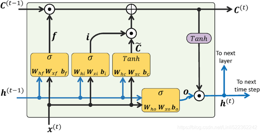

Now let’s open the box! The key idea is that the network can learn what to store in the long-term state, what to throw away, and what to read from it. As the long-term state traverses the network from left to right, you can see that it first goes through a forget gate OR , dropping some memories, and then it adds some new memories via the addition operation OR (which adds the memories that were selected by an input gate OR). The result is sent straight out, without any further transformation. So, at each time step, some memories are dropped and some memories are added. Moreover, after the addition operation, the long-term state is copied and passed through the tanh function, and then the result is filtered by the output gateOR. This produces the short-term state (which is equal to the cell’s output for this time step, ). Now let’s look at where new memories come from and how the gates work.

First, the current input vector and the previous short-term state are fed to four different fully connected layers. They all serve a different purpose:

• The main layer is the one that outputs . It has the usual role of analyzing the current inputs and the previous (short-term) state . In a basic cell, there is nothing other than this layer, and its output goes straight out to and . In contrast, in an LSTM cell this layer’s output does not go straight out, but instead its most important parts are stored in the long-term state (and the rest is dropped).
• The three other layers are gate controllers. Since they use the logistic activation function, their outputs range from 0 to 1. As you can see, their outputs are fed to element-wise multiplication operations, so if they output 0s they close the gate, and if they output 1s they open it. Specifically:
—The forget gate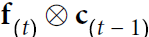 OR (controlled by ) controls which parts of the long-term state should be erased.)
(This gate decides what information should be thrown away or kept. Information from the previous hidden state and information from the current input is passed through the sigmoid function. Values come out between 0 and 1. The closer to 0 means to forget, and the closer to 1 means to keep. OR This has a possibility of dropping values in the cell state if it gets pointwise multiplied by values near 0.).
Now, is computed as follows: OR
—The input gate OR(controlled by ) controls which parts of should be added to the long-term state.)
First, we pass the previous hidden state and current input into a sigmoid function. That decides which values will be updated by transforming the values to be between 0 and 1. 0 means not important, and 1 means important. OR
You also pass the hidden state and current input into the tanh functionOR to squish values between -1 and 1 to help regulate the network.
Then you multiply the tanh output with the sigmoid output. The sigmoid output will decide which information is important to keep from the tanh output.OR.
The cell state at time t is computed as follows: OR
do a pointwise addition which updates the cell state to new values that the neural network finds relevant. That gives us our new cell state.
after the addition operation, the long-term state is copied and passed through the tanh function, and then the result is filtered by the output gate
—Finally, the output gate (controlled by ) controls which parts of the longterm state should be read and output at this time step, both to and to .
First, we pass the previous hidden state and the current input into a sigmoid function.
OR
Then we pass the newly modified cell state to the tanh function.
We multiply the tanh output with the sigmoid output to decide what information the hidden state should carry. The output is the hidden state. The new cell state and the new hidden is then carried over to the next time step.

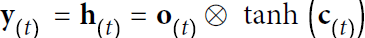
In short, an LSTM cell can learn to recognize an important input (that’s the role of the input gate), store it in the long-term state, preserve it for as long as it is needed (that’s the role of the forget gate), and extract it whenever it is needed. This explains why these cells have been amazingly successful at capturing long-term patterns in time series, long texts, audio recordings, and more.

Equation 15-3 summarizes how to compute the cell’s long-term state, its short-term state, and its output at each time step for a single instance (the equations for a whole
mini-batch are very similar).
Equation 15-3. LSTM computations https://blog.csdn.net/Linli522362242/article/details/113846940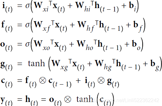

In this equation:

• , , , are the weight matrices of each of the four layers for their connection to the input vector .
• are the weight matrices of each of the four layers for their connection to the previous short-term state .
• are the bias terms for each of the four layers. Note that TensorFlow initializes to a vector full of 1s instead of 0s. This prevents forgetting everything at the beginning of training.

Peephole connections

In a regular LSTM cell, the gate controllers can look only at the input and the previous short-term state . It may be a good idea to give them a bit more context by
letting them peek at the long-term state as well. This idea was proposed by Felix Gers and Jürgen Schmidhuber in 2000.(F. A. Gers and J. Schmidhuber, “Recurrent Nets That Time and Count,” Proceedings of the IEEE-INNS-ENNS International Joint Conference on Neural Networks (2000): 189–194.) They proposed an LSTM variant with extra connections called peephole connections: the previous long-term state is added as an input to the controllers of the forget gate and the input gate, and the current longterm
state is added as input to the controller of the output gate. This often improves performance, but not always, and there is no clear pattern for which tasks are better off with or without them: you will have to try it on your task and see if it helps.

In Keras, the LSTM layer is based on the keras.layers.LSTMCell cell, which does not support peepholes. The experimental tf.keras.experimental.PeepholeLSTMCell
does, however, so you can create a keras.layers.RNN layer and pass a PeepholeLSTM Cell to its constructor.

There are many other variants of the LSTM cell. One particularly popular variant is the GRU cell, which we will look at now.

GRU cells

The Gated Recurrent Unit (GRU) cell (see Figure 15-10) was proposed by Kyunghyun Cho et al. in a 2014 paper(Kyunghyun Cho et al., “Learning Phrase Representations Using RNN Encoder-Decoder for Statistical Machine Translation,” Proceedings of the 2014 Conference on Empirical Methods in Natural Language Processing (2014): 1724–1734.) that also introduced the Encoder–Decoder network we discussed earlier.
Figure 15-10. GRU cell https://blog.csdn.net/Linli522362242/article/details/113846940
OR

Equation 15-4 summarizes how to compute the cell’s state at each time step for a single instance.
OR

Variables : The original is a sigmoid function. and : The original is a hyperbolic tangent.

: input vector
: output vector
: update gate vector ( <== input <== and ### hidden: bias )
: reset gate vector ( <== input <== and ### hidden: bias) ==> OR
OR: candidate activation vector ( <== input <==, )
W, U and b: parameter matrices and vector
If the gate controller outputs a 1, the forget gate is open (= 1, then ) and the input gate is closed (1 – 1 = 0).
If it outputs a 0, the opposite happens.

The GRU cell is a simplified version of the LSTM cell, and it seems to perform just as well (A 2015 paper by Klaus Greff et al., “LSTM: A Search Space Odyssey”, seems to show that all LSTM variants perform roughly the same.) (which explains its growing popularity). These are the main simplifications:

Left Figure:

• Both state vectors( and ) are merged into a single vector .
• A single gate(update gate) controller controls both the forget gate and the input gate
If the gate controller outputs a 1, the forget gate is open (= 1, then ) and the input gate is closed (1 – 1 = 0).
If it outputs a 0, the opposite happens.
In other words, whenever a memory must be stored, the location where it will be stored is erased first. This is actually a frequent variant to the LSTM cell in and of itself.
• There is no output gate; the full state vector is output at every time step. However, there is a new gate controller (reset gate) that controls which part of the previous state will be shown to the main layer ().

Keras provides a keras.layers.GRU layer (based on the keras.layers.GRUCell memory cell); using it is just a matter of replacing SimpleRNN or LSTM with GRU.

def generate_time_series(batch_size, n_steps):
    freq1, freq2, offsets1, offsets2 = np.random.rand(4, batch_size, 1)
    # print(freq1.shape) # (batches,1)
    time = np.linspace(0,1, n_steps) 
    # print(time.shape)  # (n_steps+1,)
    
    # https://numpy.org/doc/stable/user/basics.broadcasting.html
    # time-offsets1 shape: (n_steps+1,)-(batches,1) 
    # the axes operation is from right to left : 
    #                         time.shape(n_steps+1,)         - freq1.shape(batches,1)
    #                      ==>time.shape(,n_steps+1)         - freq1.shape(batches,1)
    # broadcast operation  ==>time.shape(batches, n_steps+1) along row(batches)
    #                         - offsets1.shape(batches,n_steps+1) along column(,n_steps+1)
    #                       result.shape(batches,n_steps+1)
    series = 0.5*np.sin( (time-offsets1)*(freq1*10 + 10) )  # wave 1 in the 1st row
    #print(series.shape) # (batches, n_steps+1)
    # += : series.extend()
    series += 0.2*np.sin( (time-offsets2)*(freq2*20 + 20) )  # +wave 2 in the 2nd row
    # print(series.shape) # (batches, n_steps+1)
    series += 0.1*(np.random.rand(batch_size, n_steps)-0.5) # +noise in the 3rd row
    # print(series.shape) # (batches, n_steps+1)
    
    return series[..., np.newaxis].astype( np.float32 )

np.random.seed(42)

n_steps = 50
series = generate_time_series(10000, n_steps+10) # 10000x60x1
X_train = series[:7000, :n_steps] # 7000x50x1
X_valid = series[7000:9000, :n_steps]
X_test = series[9000:, :n_steps]

Y = np.empty( (10000, n_steps, 10) ) #  # 10000x50x10
for step_ahead in range(1, 10+1): # Y :0     1     2          9     #[,rows=n_steps, column_index] 
    # Y[..., 0~9]                    # 1~50, 2~51, 3~52, ..., 10~59     # row range at each loop 
    Y[..., step_ahead-1] = series[..., step_ahead:step_ahead+n_steps, 0]# get 50 data at each loop

Y_train = Y[:7000]
Y_valid = Y[7000:9000]
Y_test = Y[9000:]

X_train.shape, Y_train.shape

import tensorflow as tf
from tensorflow import keras

np.random.seed(42)
tf.random.set_seed(42)

model = keras.models.Sequential([
    keras.layers.GRU(20, return_sequences=True, input_shape=[None,1]),
    keras.layers.GRU(20, return_sequences=True),
    keras.layers.TimeDistributed(keras.layers.Dense(10))
])

def last_time_step_mse( Y_true, Y_pred):  # ":" represents all instances, "-1" is last time step
    return keras.metrics.mean_squared_error( Y_true[:, -1], Y_pred[:, -1] )

model.compile(loss="mse", optimizer="adam", metrics=[last_time_step_mse])
history = model.fit(X_train, Y_train, epochs=20, validation_data=(X_valid, Y_valid))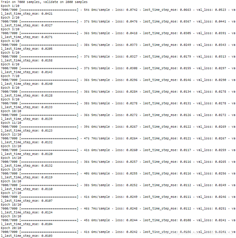

model.evaluate(X_valid, Y_valid)

import matplotlib as mpl
import matplotlib.pyplot as plt

def plot_learning_curves(loss, val_loss):
    # the validation error is computed at the end of each epoch,
    # while the training error is computed using a running mean during each epoch. 
    # So the training curve should be shifted by half an epoch to the left.
    plt.plot( np.arange( len(loss) )+0.5, loss, "b.-", label="Training loss" )
    plt.plot( np.arange( len(val_loss) )+1, val_loss, "r.-", label="Validation loss" )
    
    plt.axis([0, 20, 0, 0.05])
    plt.gca().xaxis.set_major_locator( mpl.ticker.MaxNLocator(integer=False) )
    plt.legend( fontsize=14 )
    plt.xlabel("Epochs")
    plt.ylabel("Loss")
    plt.grid(True)

plot_learning_curves(history.history["loss"], history.history["val_loss"])

plt.show()

def generate_time_series(batch_size, n_steps):
    freq1, freq2, offsets1, offsets2 = np.random.rand(4, batch_size, 1)
    # print(freq1.shape) # (batches,1)
    time = np.linspace(0,1, n_steps) 
    # print(time.shape)  # (n_steps+1,)
    
    # https://numpy.org/doc/stable/user/basics.broadcasting.html
    # time-offsets1 shape: (n_steps+1,)-(batches,1) 
    # the axes operation is from right to left : 
    #                         time.shape(n_steps+1,)         - freq1.shape(batches,1)
    #                      ==>time.shape(,n_steps+1)         - freq1.shape(batches,1)
    # broadcast operation  ==>time.shape(batches, n_steps+1) along row(batches)
    #                         - offsets1.shape(batches,n_steps+1) along column(,n_steps+1)
    #                       result.shape(batches,n_steps+1)
    series = 0.5*np.sin( (time-offsets1)*(freq1*10 + 10) )  # wave 1 in the 1st row
    #print(series.shape) # (batches, n_steps+1)
    # += : series.extend()
    series += 0.2*np.sin( (time-offsets2)*(freq2*20 + 20) )  # +wave 2 in the 2nd row
    # print(series.shape) # (batches, n_steps+1)
    series += 0.1*(np.random.rand(batch_size, n_steps)-0.5) # +noise in the 3rd row
    # print(series.shape) # (batches, n_steps+1)
    
    return series[..., np.newaxis].astype( np.float32 )

np.random.seed(43)

series = generate_time_series(1, 50+10)
X_new, Y_new = series[:, :50, :], series[:, 50:, :]
Y_pred = model.predict( X_new )[:, -1][..., np.newaxis] #-1: the last time step with features(=1),
Y_pred                               #[batch size, time steps, 1]

def plot_series( series, 
                 y=None, 
                 y_pred=None, 
                 x_label="$t$", y_label="$x(t)$" 
               ):
    plt.plot( series, ".-")
    if y is not None:
        plt.plot( n_steps, y, "bx", markersize=10)
    if y_pred is not None:
        plt.plot( n_steps, y_pred, "ro", markersize=10)
        
    if x_label:
        plt.xlabel(x_label, fontsize=16)
    if y_label:
        plt.ylabel(y_label, fontsize=16, labelpad=15, rotation=0)

    plt.hlines(0, 0, n_steps+1, linewidth=1)
    plt.axis([0, n_steps+1, -1, 1])
    plt.grid(True)

def plot_multiple_forecasts( X,Y,Y_pred):
    n_steps = X.shape[1]
    ahead = Y.shape[1]
    
    plot_series(X[0, :, 0]) # first series in X
    plt.plot( np.arange(n_steps, n_steps+ahead), Y[0, :, 0],
              "yo-", label="Actual" )
    plt.plot( np.arange(n_steps, n_steps+ahead), Y_pred[0, :, 0],
              "bx-", label="Forecast", markersize=10 )
    
    plt.axis([0, n_steps+ahead, -1, 1])
    plt.legend( fontsize=14 )
    
plot_multiple_forecasts(X_new, Y_new, Y_pred)

plt.show()

LSTM and GRU cells are one of the main reasons behind the success of RNNs. Yet while they can tackle much longer sequences than simple RNNs, they still have a
fairly limited short-term memory, and they have a hard time learning long-term patterns in sequences of 100 time steps or more, such as audio samples, long time series, or long sentences. One way to solve this is to shorten the input sequences, for example using 1D convolutional layers.

Using 1D convolutional layers to process sequences

https://blog.csdn.net/Linli522362242/article/details/115258834

15_RNN_naive_linear_CNN预测顺序数据10值_scalar_plt.sca_labelpad_curve_Layer Normal_TimeDistributed_LSTM_GRU