Boole‘s，Doob‘s inequality，中心极限定理Central Limit Theorem，Kolmogorov extension theorem, Lebesgue‘s domin

1. Boole’s inequality

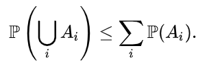
In probability theory, Boole’s inequality, also known as the union bound, says that for any finite or countable set of events, the probability that at least one of the events happens is no greater than the sum of the probabilities of the individual events.

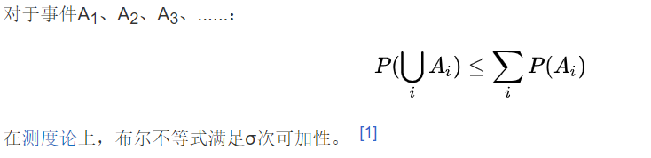
布尔不等式（Boole’s inequality），由乔治·布尔提出，指对于全部事件的概率不大于单个事件的概率总和。

Formally, for a countable set of events A1, A2, A3, …, we have
在这里插入图片描述

在这里插入图片描述

1.1 Proof using induction

在这里插入图片描述

1.2 Proof without using induction

在这里插入图片描述

1.3 Generalization

Boole’s inequality may be generalized to find upper and lower bounds on the probability of finite unions of events. These bounds are known as Bonferroni inequalities, after Carlo Emilio Bonferroni;
在这里插入图片描述
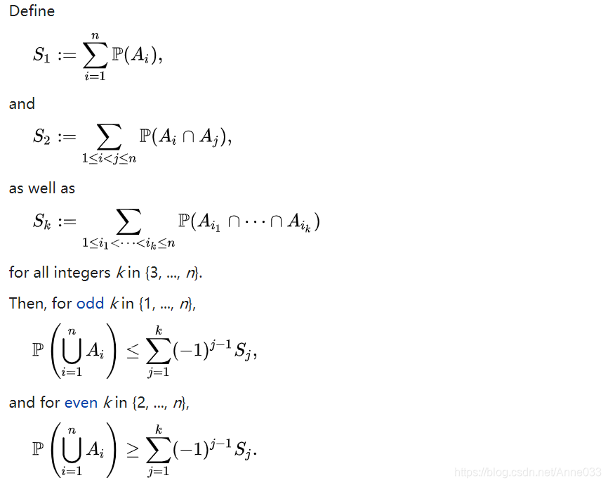
Boole’s inequality is the initial case, k = 1. When k = n, then equality holds and the resulting identity is the inclusion–exclusion principle.

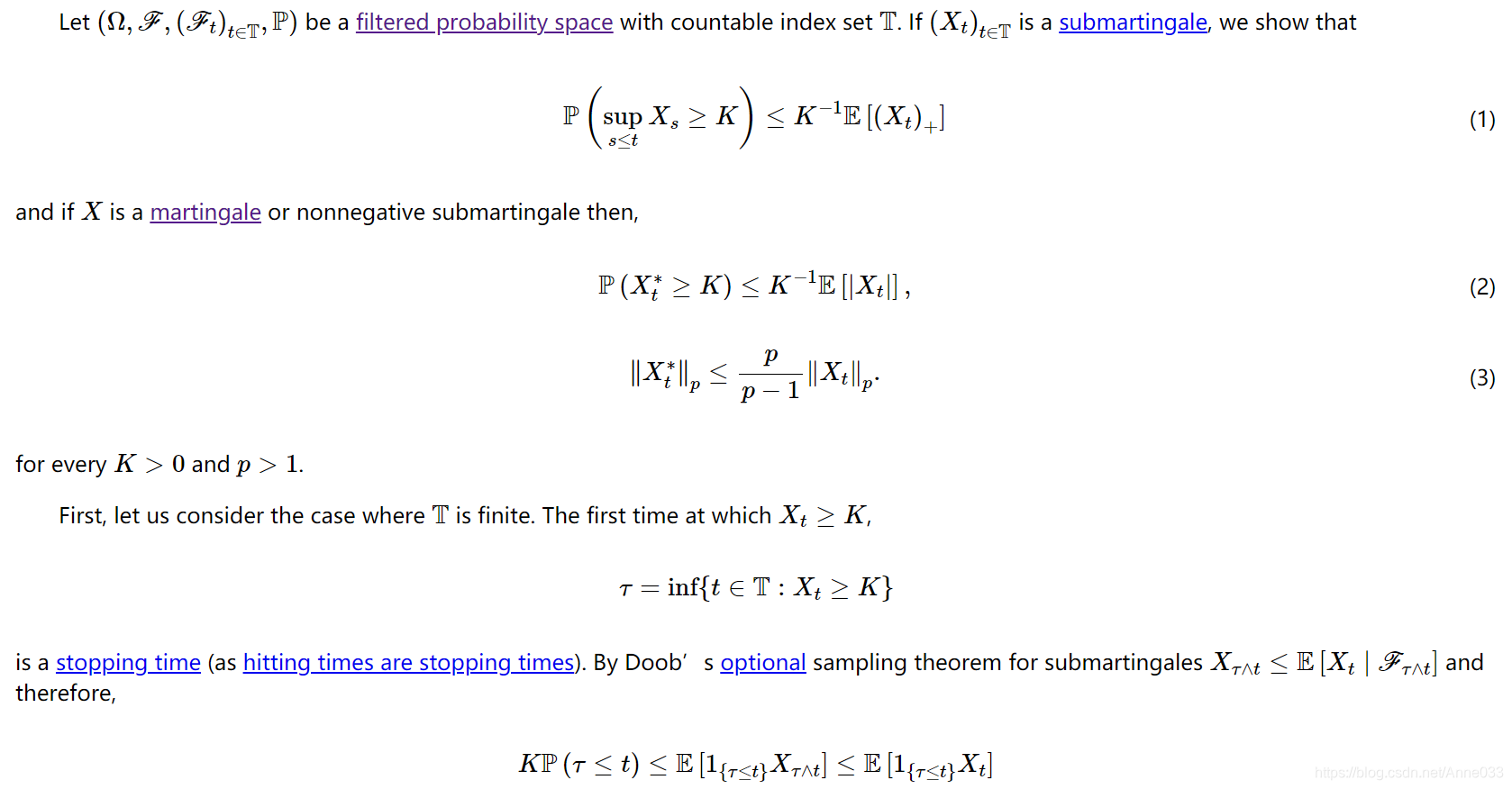
2. Doob’s inequality

在这里插入图片描述

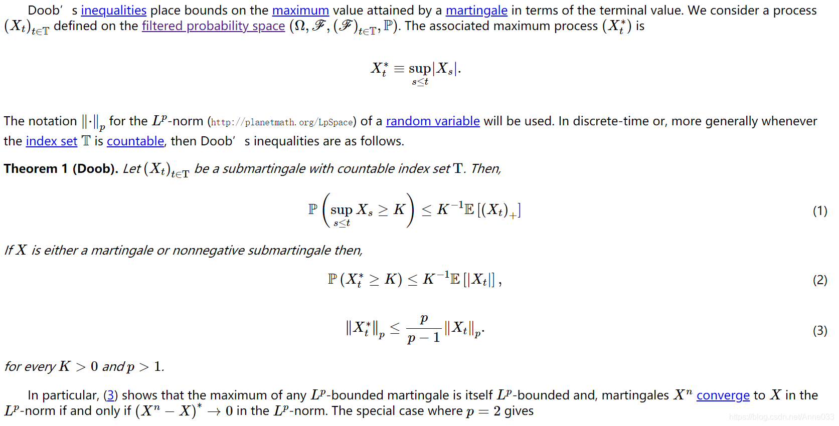
for every K>0 and p>1.

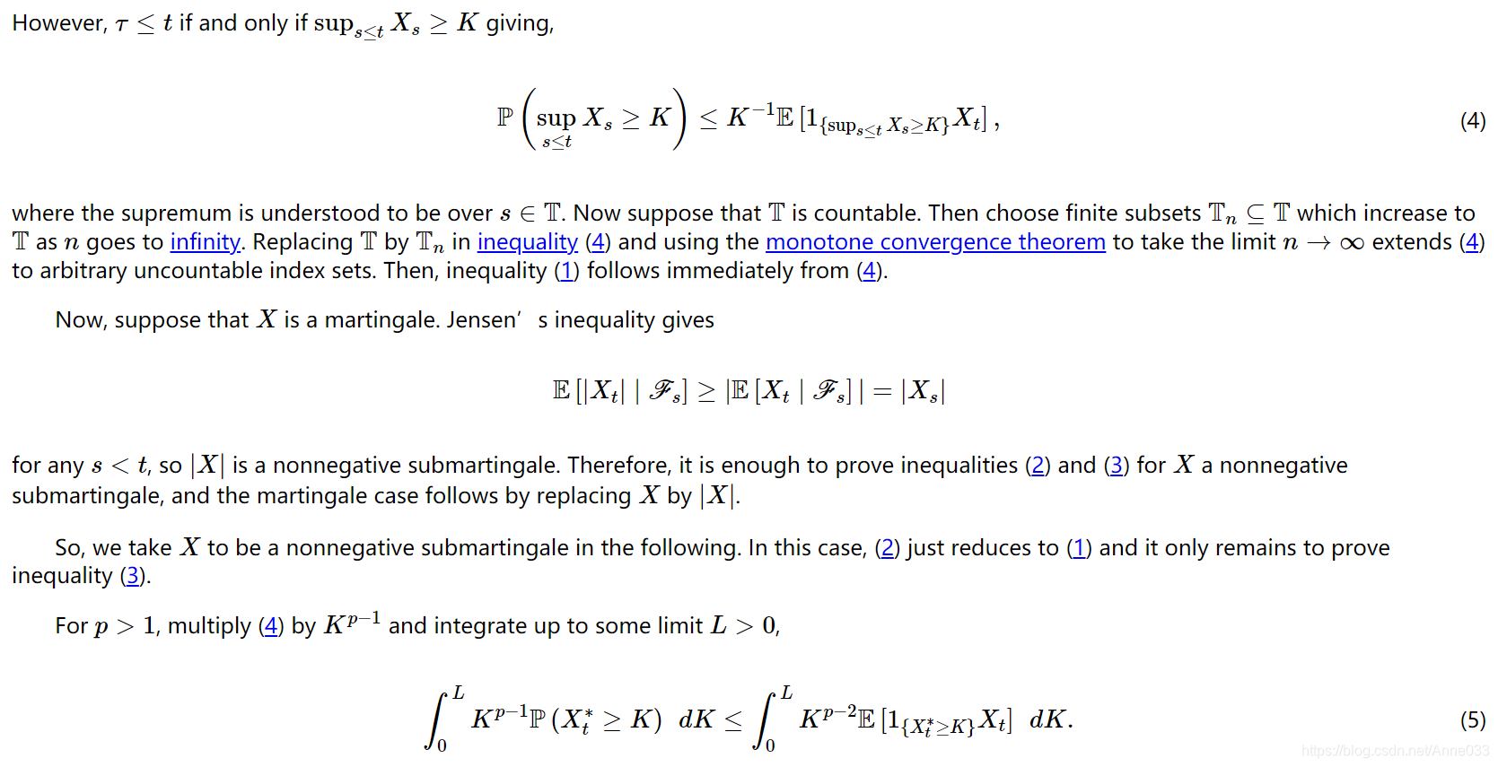
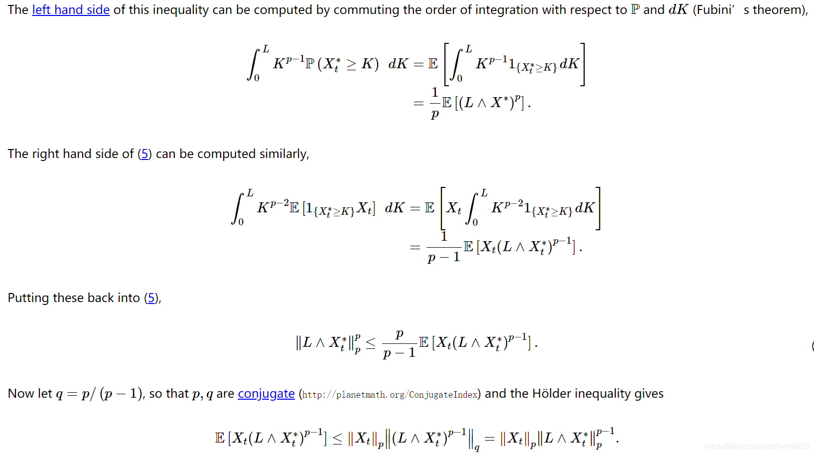
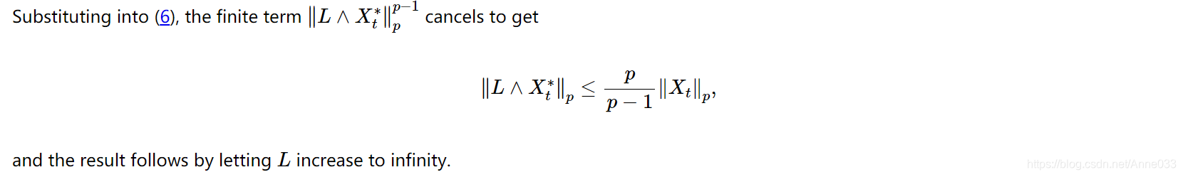
2.1 proof of Doob’s inequalities

在这里插入图片描述

3. 中心极限定理（Central Limit Theorem）

中心极限定理指的是给定一个任意分布的总体。我每次从这些总体中随机抽取 n 个抽样，一共抽 m 次。然后把这 m 组抽样分别求出平均值。这些平均值的分布接近正态分布。

我们先举个栗子?

现在我们要统计全国的人的体重，看看我国平均体重是多少。当然，我们把全国所有人的体重都调查一遍是不现实的。所以我们打算一共调查1000组，每组50个人。然后，我们求出第一组的体重平均值、第二组的体重平均值，一直到最后一组的体重平均值。中心极限定理说：这些平均值是呈现正态分布的。并且，随着组数的增加，效果会越好。最后，当我们再把1000组算出来的平均值加起来取个平均值，这个平均值会接近全国平均体重。

其中要注意的几点：

总体本身的分布不要求正态分布
上面的例子中，人的体重是正态分布的。但如果我们的例子是掷一个骰子（平均分布），最后每组的平均值也会组成一个正态分布。（神奇！）
样本每组要足够大，但也不需要太大
取样本的时候，一般认为，每组大于等于30个，即可让中心极限定理发挥作用。

中心极限定理也就是这么两句话：
1）任何一个样本的平均值将会约等于其所在总体的平均值。
2）不管总体是什么分布，任意一个总体的样本平均值都会围绕在总体的平均值周围，并且呈正态分布。

在这里插入图片描述

在实际生活当中，我们不能知道我们想要研究的对象的平均值，标准差之类的统计参数。中心极限定理在理论上保证了我们可以用只抽样一部分的方法，达到推测研究对象统计参数的目的。

3.1 中心极限定理有什么用呢？

1）在没有办法得到总体全部数据的情况下，我们可以用样本来估计总体如果我们掌握了某个正确抽取样本的平均值和标准差，就能对估计出总体的平均值和标准差。举个例子，如果你是北京西城区的领导，想要对西城区里的各个学校进行教学质量考核。同时，你并不相信各个学校的的统考成绩，因此就有必要对每所学校进行抽样测试，也就是随机抽取100名学生参加一场类似统考的测验。作为主管教育的领导，你觉得仅参考100名学生的成绩就对整所学校的教学质量做出判断是可行的吗？答案是可行的。中心极限定理告诉我们，一个正确抽取的样本不会与其所代表的群体产生较大差异。也就是说，样本结果（随机抽取的100名学生的考试成绩）能够很好地体现整个群体的情况（某所学校全体学生的测试表现）。当然，这也是民意测验的运行机制所在。通过一套完善的样本抽取方案所选取的1200名美国人能够在很大程度上告诉我们整个国家的人民此刻正在想什么。2）根据总体的平均值和标准差，判断某个样本是否属于总体如果我们掌握了某个总体的具体信息，以及某个样本的数据，就能推理出该样本是否就是该群体的样本之一。通过中心极限定理的正态分布，我们就能计算出某个样本属于总体的概率是多少。如果概率非常低，那么我们就能自信满满地说该样本不属于该群体。

大数定律https://www.zhihu.com/question/19911209/answer/245487255

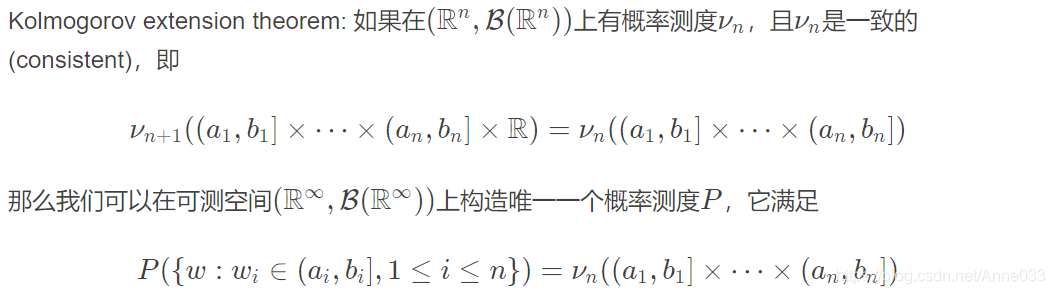
4. Kolmogorov extension theorem

In mathematics, the Kolmogorov extension theorem (also known as Kolmogorov existence theorem, the Kolmogorov consistency theorem or the Daniell-Kolmogorov theorem) is a theorem that guarantees that a suitably “consistent” collection of finite-dimensional distributions will define a stochastic process. It is credited to the English mathematician Percy John Daniell and the Russian mathematician Andrey Nikolaevich Kolmogorov.

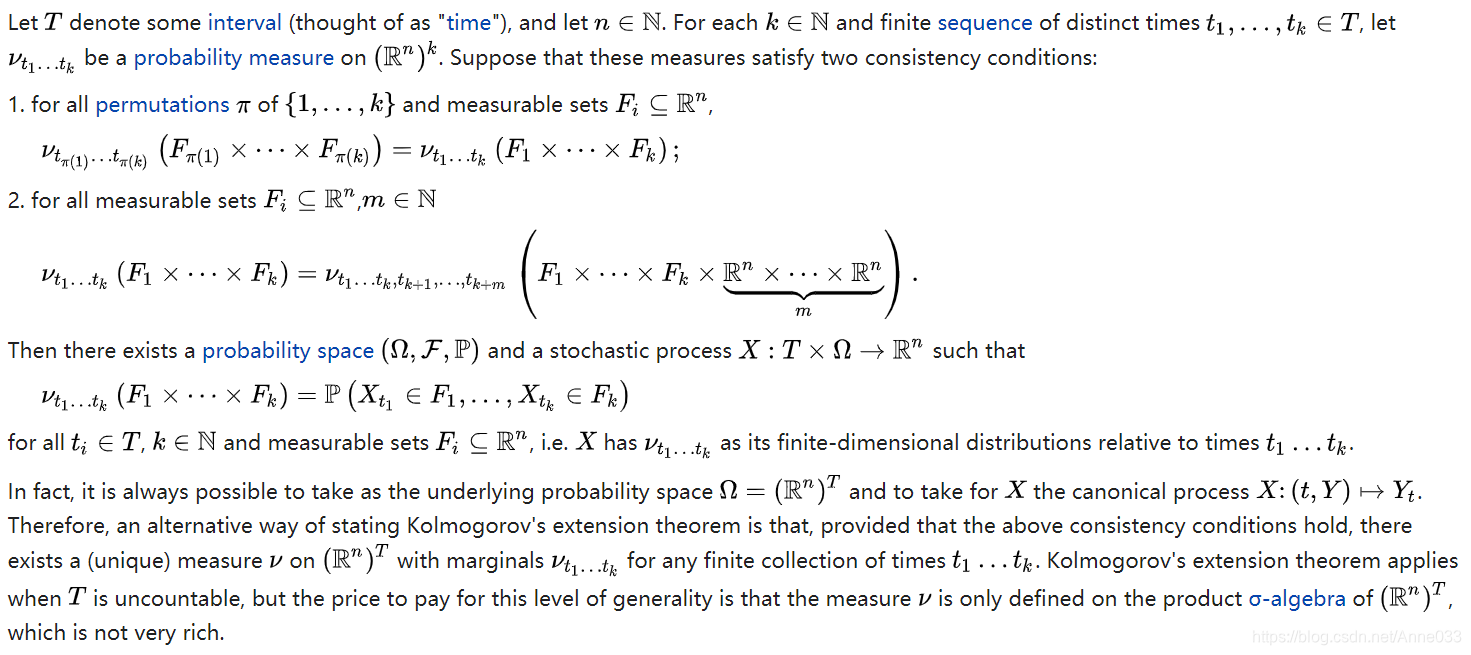
4.1 Statement of the theorem

在这里插入图片描述

In fact, it is always possible to take as the underlying probability space $\Omega =(\mathbb {R} ^{n})^{T}$ and to take for $X$ the canonical process $X\colon (t,Y)\mapsto Y_{t}$ . Therefore, an alternative way of stating Kolmogorov’s extension theorem is that, provided that the above consistency conditions hold, there exists a (unique) measure $\nu$ on $(\mathbb {R} ^{n})^{T}$ with marginals $\nu _{t_{1}\dots t_{k}}$ for any finite collection of times $t_{1}\dots t_{k}$ . Kolmogorov’s extension theorem applies when $T$ is uncountable, but the price to pay for this level of generality is that the measure $\nu$ is only defined on the product σ-algebra of $(\mathbb {R} ^{n})^{T}$ , which is not very rich.

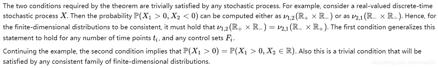
4.2 Explanation of the conditions

在这里插入图片描述

4.3 Implications of the theorem

Since the two conditions are trivially satisfied for any stochastic process, the power of the theorem is that no other conditions are required: For any reasonable (i.e., consistent) family of finite-dimensional distributions, there exists a stochastic process with these distributions.

The measure-theoretic approach to stochastic processes starts with a probability space and defines a stochastic process as a family of functions on this probability space. However, in many applications the starting point is really the finite-dimensional distributions of the stochastic process. The theorem says that provided the finite-dimensional distributions satisfy the obvious consistency requirements, one can always identify a probability space to match the purpose. In many situations, this means that one does not have to be explicit about what the probability space is. Many texts on stochastic processes do, indeed, assume a probability space but never state explicitly what it is.

The theorem is used in one of the standard proofs of existence of a Brownian motion, by specifying the finite dimensional distributions to be Gaussian random variables, satisfying the consistency conditions above. As in most of the definitions of Brownian motion it is required that the sample paths are continuous almost surely, and one then uses the Kolmogorov continuity theorem to construct a continuous modification of the process constructed by the Kolmogorov extension theorem.

4.4 General form of the theorem

The Kolmogorov extension theorem gives us conditions for a collection of measures on Euclidean spaces to be the finite-dimensional distributions of some $\mathbb {R} ^{n}$ -valued stochastic process, but the assumption that the state space be $\mathbb {R} ^{n}$ is unnecessary. In fact, any collection of measurable spaces together with a collection of inner regular measures defined on the finite products of these spaces would suffice, provided that these measures satisfy a certain compatibility relation. The formal statement of the general theorem is as follows.

This theorem has many far-reaching consequences; for example it can be used to prove the existence of the following, among others:

Brownian motion, i.e., the Wiener process,
a Markov chain taking values in a given state space with a given transition matrix,
infinite products of (inner-regular) probability spaces.

4.5 History

According to John Aldrich, the theorem was independently discovered by British mathematician Percy John Daniell in the slightly different setting of integration theory.

在这里插入图片描述

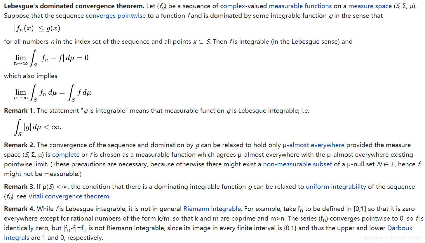
5. Lebesgue’s dominated convergence theorem

In measure theory, Lebesgue’s dominated convergence theorem provides sufficient conditions under which almost everywhere convergence of a sequence of functions implies convergence in the L1 norm. Its power and utility are two of the primary theoretical advantages of Lebesgue integration over Riemann integration.

In addition to its frequent appearance in mathematical analysis and partial differential equations, it is widely used in probability theory, since it gives a sufficient condition for the convergence of expected values of random variables.

5.1 Statement

在这里插入图片描述

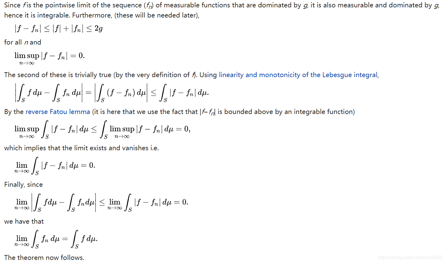
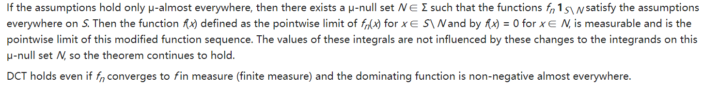
5.2 Proof

Without loss of generality, one can assume that f is real, because one can split f into its real and imaginary parts (remember that a sequence of complex numbers converges if and only if both its real and imaginary counterparts converge) and apply the triangle inequality at the end.

Lebesgue’s dominated convergence theorem is a special case of the Fatou–Lebesgue theorem. Below, however, is a direct proof that uses Fatou’s lemma as the essential tool.
在这里插入图片描述

https://en.wikipedia.org/wiki/Boole%27s_inequality
https://planetmath.org/alphabetical.html
https://zhuanlan.zhihu.com/p/25241653
https://www.zhihu.com/question/22913867
https://en.wikipedia.org/wiki/Kolmogorov_extension_theorem
https://blog.csdn.net/weixin_44207974/article/details/111503988
https://blog.csdn.net/weixin_44207974/article/details/111602960
https://en.wikipedia.org/wiki/Dominated_convergence_theorem