PLONK: permutations over lagrange-bases for oecumenical noninteractive arguments of knowledge 学习笔记

1. 引言

Gabizon等人2019年论文《PLONK: permutations over lagrange-bases for oecumenical noninteractive arguments of knowledge》。

相关代码实现有：

• https://github.com/dusk-network/plonk
• https://github.com/barryWhiteHat/plonk_tutorial
• https://github.com/mir-protocol/plonky
• https://github.com/matter-labs/solidity_plonk_verifier
• https://github.com/matter-labs/recursive_aggregation_circuit
• https://github.com/dusk-network/plonk_gadgets
• https://github.com/dusk-network/dusk-blindbid
• https://github.com/Fluidex/awesome-plonk
• https://github.com/Fluidex/plonkit
• https://github.com/zcash/halo2

---

要点：
（1）与Spartan 中将R1CS中的A/B/C 分别以multilinear多项式表示不同，Plonk中是将circuit中所有门的左侧、右侧和输出分别以多项式$f_L,f_R,f_O$表示。
（2）[BG12]《Efficient zero-knowledge argument for correctness of a shuffle》中的 permutation argument的核心思路为构建双变量多项式：
${\prod }_{i=1}^N(d_i-z)={\prod }_{i=1}^N(yi+x^i-z)$
利用product argument证明以上关系成立，即完成相应的permutation argument（又称为shuffle argument）。
而Plonk中，是基于lagrange-bases构建的单变量多项式，如test_permutation_compute_sigmas_only_left_wires()测试用例中所示，${\sigma }_0,{\sigma }_1,{\sigma }_2,{\sigma }_3$多项式对应的点值表示满足相应的permutation关系即可：【对应为单变量多项式。】
${\prod }_{i=0}^N(w{l}_i+\beta {\omega }^i+\gamma )(w{r}_i+\beta {\omega }^i+\gamma )(w{o}_i+\beta {\omega }^i+\gamma )(w{4}_i+\beta {\omega }^i+\gamma )={\prod }_{i=0}^N(w{l}_i+\beta {\sigma }_0({\omega }^i)+\gamma )(w{r}_i+\beta {\sigma }_1({\omega }^i)+\gamma )(w{o}_i+\beta {\sigma }_2({\omega }^i)+\gamma )(w{4}_i+\beta {\sigma }_3({\omega }^i)+\gamma )$
circuit wire与${\sigma }_i$之间的permutation关系很巧妙，具体见compute_sigma_permutations()函数。

---

1）Groth等人2018年论文[GKM+]《 Updatable and universal common reference strings with applications to zk-snarks》，在构建zk-SNARK过程中引入了updatable structured reference string (SRS)，扫除了zk-SNARKs实际部署时的一个主要障碍。
2）Maller等人2019年论文[MBKM19]《 Sonic: Zeroknowledge snarks from linear-size universal and updateable structured reference strings》，是第一个可能实用的zk-SNARK，具有fully succinct verification for general arithmetic circuits with such an SRS。但是为了实现fully succinct verification，Sonic方案中构建proof的开销仍然很大。

本文构建的 universal SNARK，具有：

• fully succinct verification
• significantly lower prover running time （fully succinct verifier模式下，group exponentiations的计算量比[MBKM19]少7.5~20倍（具体取决于具体的circuit结构））

与[MBKM19]类似，本文的实现也依赖于 Bayer和Groth 2012年论文[BG12]《Efficient zero-knowledge argument for correctness of a shuffle》中的 permutation argument。【可参见本人系列博客：

• Efficient Zero-Knowledge Argument for Correctness of a Shuffle学习笔记（1）
• Efficient Zero-Knowledge Argument for Correctness of a Shuffle学习笔记（2）
• Efficient Zero-Knowledge Argument for Correctness of a Shuffle学习笔记（3）】

但是，本文专注于 “Evaluations on a subgroup” 而不是 “coefficients of monomials”，因此可简化相应的permutation argument 和 the arithmetization step。

1.1 背景介绍

考虑到zk-SNARKs的实际部署，人们开始关注 可提供 “universal and updatable” 的structured reference string (SRS) 模式。
SRS可用于：

• statements about all circuits of a certain bounded size;
• 在任意时间点，SRS可由新的参与方更新，使得在该时间点的所有updaters中只要由一方是honest的，就可保证整个算法的soundness。

为了简化，本文称具有SRS setup的zk-SNARK为universal的。

同时，若zk-SNARK for circuit satisfiablity 满足以下条件，可称其为fully succinct的：

• 1）preprocessing phase或SRS generation 的run time为quasilinear in circuit size。【其中preprocessing 是指如 [GGPR13] Gennaro等人2013年论文《Quadratic span programs and succinct nizks without pcps》中，允许one-time verifier computation that is polynomial rather than polylogarithmic in the circuit size，从而使得SNARK可用于所有non-uniform circuits，而不仅适于statements about uniform computation。】
• 2）Prover 的 run time为quasilinear in circuit size。
• 3）Proof length为logarithmic in circuit size。【理论上讲，polylogarithmic proof length更自然，但是logarithmic非常好的实现了constant number of group elements，很好的契合了实际使用需求。】
• 4）Verifier 的 run time为polylogarithmic in circuit size。【在很多定义中，仅要求proof size为polylogarithmic，如[GGPR13]中的术语中，若要求proof size为polylogarithmic的同时还要求verifier的run time为polylogarithmic，这样的SNARK是不存在的。】

Maller等人2019年论文[MBKM19]《 Sonic: Zeroknowledge snarks from linear-size universal and updateable structured reference strings》中，第一次实现了a universal fully succinct zk-SNARK for circuit satisfiability——Sonic。
同时在该论文中，提供了Sonic的一个改进版本，可大幅改进Prover的run time，代价是 efficient verification only in a certain amortized sense。

1.2 我们的成果

相比于fully-succint Sonic，我们显著改善了Prover run time。
改进的主要点在于：

• 相比于[BCC+16] Bootle等人2016年《Efficient zero-knowledge arguments for arithmetic circuits in the discrete log setting》，受[MBKM19]中的计算启发，实现了更直接的arithmetization of a circuit。将 permuataion argument 与 单变量evaluations on a multiplicative subgroup 结合，而不是 [MBKM19]中的 coefficients of 双变量多项式。【具体可见本文博客 Efficient Zero-Knowledge Arguments for Arithmetic Circuits in the Discrete Log Setting学习笔记】

简而言之，合理的multiplicative subgroups在很多协议中都很实用，包括Sonic——使用了[BG12]中的permutation argument。
最终，在“grand product argument”中，可reduce为check relations between coefficients of polynomials at “neighbouring monomials”。

若将 $x,g\cdot x$看成是neighbour points对，其中$g$为generator of a multiplicative subgroup of a field $\mathbb{F}$，则将很容易检查不同曲线在这些points对的关系。
还有一个便捷之处是，multiplicative subgroups可与Lagrange bases进行良好交互。如，若$H\subset \mathbb{F}$ 为a multiplicative subgroup of order $n+1$，且$x\in H$，则多项式$L_x$ of degree at most $n$ that vanishes on H ∖ { x } H\setminus\{x\} H∖{ x} and has $f(x)=1$可以非常稀疏的方式表示为：【因为$X\in H$，而$H$的order为$n+1$，因此有$X^{n+1}=1$。】
$L_x(X)=\frac{c_x(X^{n+1}-1)}{X-x}$
其中$c_x$为常数。
当构建efficiently verifiable [BG12]-形式 的permutation argument时，以这种多项式identities方式表示将是有益的。

1.3 效率分析

将本文的研究成果与现有的non-universal SNARKs和universal SNARKs进行了性能对比。

• 在本文发表时，仅有[MBKM19]的Sonic protocol是fully succinct universal SNARK，Sonic protocol需要做 $273n$ 次 ${\mathbb{G}}_1$ group exponentiations运算，其中$n$为乘法门的数量。
  在fully-succinct Sonic中，每根线仅可表示三种线性关系，需要额外的“dummy”乘法门来容纳多余三个加法门的线。这将导致乘法门数量的增加，进而会影响Prover的computation estimate。具体可参看[MBKM19]中的详细描述。

• 而本文的universal SNARK需要Prover计算6个polynomial commitments 以及2个opening proofs to evaluate the polynomial commitments at a random challenge point。
  Plonk提供了两种模式供用户使用：proof size中增加2个group elements的化，则Prover的总计算量可降低约10%。
  The combined degree of the polynomials要么是$9(n+a)$（对应larger proofs），要么是$11(n+a)$（对应smaller proofs, reduced verifier work）。其中$n$为乘法门的数量，$a$为加法门的数量。

• [Gro16] Groth 2016年论文《 On the size of pairing-based non-interactive arguments》 是当前效率最高fully-succinct SNARK，尽管其需要unique, non-updatable CRS per circuit。[Gro16] 中构建proof的计算量主要有 $3n+m$次 ${\mathbb{G}}_1$ group expoentiations 和 $n$次${\mathbb{G}}_2$ group exponentiations组成，其中$m$为R1CS的变量数，$m$的上限值为$n$，为简化表述，可假设$m=n$。
  若假设1次${\mathbb{G}}_2$ exponentiation计算量相当于$3$次${\mathbb{G}}_1$ exponentiation计算量，则[Gro16]总的计算量相当于$6n+m$次${\mathbb{G}}_1$ group exponetiations计算量。

不过在对这些SNARK方案进行对比之前，需对一些主观假设达成共识。当evaluate common circuits时，其加法门的数量为乘法门数量的两倍，但是，若在某些假设场景下对circuit进行优化，使其不存在加法门时（常见于[Gro16]之类构建的R1CS），其评估表现将更差：【注意，以下对比都是基于所需group exponentiations计算数量。】

• 如极端情况下，对于无加法门，且仅有fan-in-2 乘法门的circuit，本文的universal SNARK proof将需要比[Gro16]多约1.1倍的prover work，而比Sonic少约30倍的prover work。
• 若$a=2n$，即加法门数量为乘法门数量的2倍时，本文的universal SNARK proof需要比[Gro16]多约2.25倍的prover work，需要比Sonic少约10倍的prover work。
• 若$a=5n$，即加法门数量为乘法门数量的5倍时，本文的universal SNARK proof需要比[Gro16]多约3倍的prover work，需要比Sonic少约5倍的prover work。

同时，在fast模式下，Plonk中structured reference string的degree与circuit中门数量相等，其SRS size实现了有效reduction。

当对比proof construction时，由于构建proof中所需的FFT数量是non-trivial的，因此还考虑Plonk中的field multiplications数量。
其它的succint universal SNARK也需要较高的FFT计算开销，考虑到这些开销不易对比，因此在下图中，未包含关于FFT的计算开销对比：

有定性分析指出，FFT的开销略低于${\mathbb{G}}_1$ group exponentiations开销。

而Verifier对每个proof的验证开销对比如下图所示：【基于the simple strucuture of the committed prover polynomials，实际Verifier仅需要2次bilinear pairing 运算。此外，每次pairing计算中的${\mathbb{G}}_2$元素是固定的，因此可通过[CS10] Costello等人2010年论文《Fixed argument pairings》 的方案进行优化，实现reduce pairing computation time by 约30%。】

实际基于BN254曲线的性能bench为：

甚至对于百万级门数量的circuit，Plonk可在消费者级别的硬件设备上在23秒内生成相应的proof。这大幅改进了universal SNARKs的效率，使其可广泛用于实际各种用户场景下。

circuit preprcessing为一次性计算，实现将每个program 编码成 一个Plonk circuit。在该步骤中，将生成polynomial commitments to the “selector” polynomials required to verify proofs。

当构建proofs时，计算FFT所需的时间 与 进行elliptic curve scalar multiplications的时间 是相当的。上表1中的field multiplication数量是从8次 FFT of size $4n$、5次 FFT of size $2n$ 以及 $12$次 FFT of size $n$ 中提取的。

当cicuit的preprocessed polynomials are provided as evaluations over the $4n$'th root of unity (而不是Lagrange-base form)时，$FFT$运算数量可进一步reduce，但是这将大幅增加构建proof所需的信息量，因此在本文的benchmark中未考虑该优化。

1.4 同期研究成果对比——randomized sumcheck方案、Fractal/Marlin

粗略地说，所有的succinct proving system都是通过使用randomness来将多个constraint check压缩为1个。常见的压缩做法是：take a random linear combination of the constraints。

在R1CS和其它类似系统中，待压缩的相对较困难的contraints为：
linear relations between the system variables，即形如$<{\vec{a}}_i,\vec{x}>=0$的contraints，其中$\vec{x}\in {\mathbb{F}}^m$为系统变量，${\vec{a}}_i\in {\mathbb{F}}^m$表示其中的一个constraint。

这类似于circuit satisifiability statement中形如$x_i=x_j$的“wiring constraints”，如$x_i$表示gate $G$的输出线，$x_j$表示由gate $G$到另一个gate $G^{\prime }$的输入线。

A random linear combination of linear constraint的形式为：
${\sum }_{i\in [n]}{r}^i<{\vec{a}}_i,\vec{x}>=0$
其中$r\in \mathbb{F}$。

忽略一些技术细节，在[MBKM19]和后续的[Gab19] Gabizon 2019年论文《Auroralight:improved prover efficiency and SRS size in a soniclike system》【基于[BCR+19] Ben-Sasson等人2018年论文《 Aurora: Transparent succinct arguments for R1CS》】将上述check reduce为 evaluate a degree $n$ bivariate $S$ at a random point，使得$S$的非零单项式数量与contraint vectors { a ⃗ i } i ∈ [ n ] \{\vec{a}_i\}_{i\in[n]} { a i​}i∈[n]​ 中的非零元素数相等。在这方面，[MBKM19]采用了更聪明的策略来amortize the cost of many evaluations of $S$ across many proofs。[MBKM19]中的方式Prover效率更高，但是无法实现fully succinct，因为需要Verifier自身来计算至少1个evaluation of $S$。

阻碍Sonic（以及[Gab19]）具有more prover efficiency + fully succinct 属性的技术难点在于：
需要一种方法来实现efficiently verify an evaluation $S(z,y)$ in the case $S$ 仅包含$O(n)$个 non-zero 单项式。

在最近同期的研究成果中，采用的解决方案为借助“Lagrange Basis”：

• Fractal：[COS19] Chiesa等人2019年论文《Fractal: Post-quantum and transparent recursive proofs from holography》。Fractal 针对的是transparent recursive SNARKs，使用的是sparse bi-variate evaluation技术。
• Marlin：[CHM+19] Chiesa等人2019年论文《Marlin: Preprocessing zksnarks with universal and updatable SRS》。Marlin 关注的是实现fully succinct (universal) SNARK，与本论文的目标一致。

特别地，假设$H,K$为multiplicative subgroups of size $O(n)$ of $\mathbb{F}$，使得$S$仅有$M$个非零值 on $H\times K$；然后[CHM+19]和[COS19]中制定了一种协议来 convince a succinct verifier that $S(z,y)=t$ where the prover’s work is linear in $M$。解决该问题的一个直观做法是将[KZG10] Kate等人2010年论文《Constant-size commitments to polynomials and their applications》 generalize为 a bi-variate polynomial commitment scheme，这将需要$O(n^2)$ proving time。

回到Plonk，不需要 “bi-variate evaluation breakthrough” 的主要原因是，Plonk关注的是constant fan-in circuits，而不是R1CS/unlimited addition fan-in。因此Plonk中的linear constraints仅仅是wiring contraints，这些wiring constraints可reduce为a permutation check（具体见本论文第5.2和6章）。

可将[BG12]中的技术理解为：
“linear constraints that correspond to a permutation can be more simply combined than general linear constraints”。
比如，在上述方程式中，每个constraint乘以不同的random coefficient；而在[BG12]的randomization中，在某种意义上，为每个变量值添加相同的random shift就足够了。（详细的permutation protocol见本论文第5章。）

本文的目标和[CHM+19] Marlin的研究目标都是：
fully succinct (universal) SNARK

但是，目前并没有完全直接的方式来对比Plonk和Marlin，原因在于Plonk在具体常熟领域，且两者所使用的basic measure 是不同的。
Plonk中的参数$n$表示的是fan-in two circuit中的加法和乘法门数量；
Marlin中的主要参数为：the maximal number of non-zeros in one of the three matrices describing an R1CS。

对于相同的$n$，Plonk的表现优于Marlin，如Prover 的group运算和proof size都将改进2倍。极端情况下，对于只有乘法门的circuit，这将代表Plonk和Marlin的性能表现差异。

但是，对于具有 “frequent large addtion fan-in” constraint system，Marlin的表现将优于 the currently specified variant of Plonk。比如，对于极端情况下的 “fully dense” R1CS constraint：
$({\sum }_{j\in [m]}{a}_j{x}_j)\cdot ({\sum }_{j\in [m]}{b}_j{x}_j)={\sum }_{j\in [m]}{c}_j{x}_j$
其中$\vec{a},\vec{b},\vec{c}\in {\mathbb{F}}^m$具有all non-zero entries。（所有元素均为非零值。）

另外，似乎将Fractal中隐含的思想——上述提及的sparse bi-variate evaluation protocol 嵌入到[Gab19]中，将改进其性能表现，特别是针对可将某些Prover work委托给外部helper的场景。而在Plonk中，不大有机会存在这样的委托，因为Plonk中的wiring is checked on the witness itself，而在[Gab19][CHM+19][COS19] 中，it is in sense checked on the random coefficients of the verifier。

2. 相关术语及约定

2.1 术语

假设field $\mathbb{F}$具有prime order。假设所有的算法中都包含了一个隐含的安全参数$\lambda$。

• ${\mathbb{F}}_{<d}[X]$ 表示的是一系列单变量多项式over $\mathbb{F}$ of degree smaller than $d$。

• efficient：是指算法的run time为$poly(\lambda )$。

• object generator $\mathcal{O}$：输入为$\lambda$，且在所有协议运行前执行。输出为all fields and groups used。
  本文 $\mathcal{O}(\lambda )=(\mathbb{F},{\mathbb{G}}_1,{\mathbb{G}}_2,{\mathbb{G}}_t,e,g_1,g_2,g_t)$，其中：
  1）$\mathbb{F}$为prime filed，具有super-polynomial size $r={\lambda }^{w(1)}$。
  2）${\mathbb{G}}_1,{\mathbb{G}}_2,{\mathbb{G}}_t$均为groups of size $r$，$e$为an efficiently computable non-degenerate pairing $e:{\mathbb{G}}_1\times {\mathbb{G}}_2\to {\mathbb{G}}_t$。
  3）$g_1,g_2$为uniformly chosen generators 使得$e(g_1,g_2)=g_t$。
  通常$\lambda$参数为隐性的，即用$\mathbb{F}$来代替$\mathbb{F}(\lambda )$。
  ${\mathbb{G}}_1$和${\mathbb{G}}_2$为加法group，具有：
  $[x{]}_1:=x\cdot g_1$
  $[x{]}_2:=x\cdot g_2$

• $[n]$表示整数 { 1 , ⋯   , n } \{1,\cdots,n\} { 1,⋯,n}

• e.w.p：全称为“except with probability”，即 e.w.p $\lambda$ 表示 probability at least $1-\lambda$。

• universal SRS-based public-coin protocols：是指可借助Fiat-Shamir transform或a random oracle 来实现non-interactive protocols。
  proof length是指the total communication of the prover。
  本文的SRS可源于：
  deterministic $poly(\lambda )$-time from an “SRS of monomials” of the form { [ x i ] 1 } a ≤ i ≤ b , { [ x i ] 2 } c ≤ i ≤ d \{[x^i]_1\}_{a\leq i\leq b}, \{[x^i]_2\}_{c\leq i\leq d} { [xi]1​}a≤i≤b​,{ [xi]2​}c≤i≤d​ for uniform $x\in \mathbb{F}$, and some integers $a,b,c,d$ with absolute value bounded by $poly(\lambda )$。
  然后遵循[BGM17] Bowe等人2017年论文《Scalable multi-party computation for zksnark parameters in the random beacon model》中要求SRS can be derived in a universal and updatable setup 仅需one honest participant —— 即若adversary控制了all but one of the participants in the setup does not gain more than a $negl(\lambda )$ advantage in its probability of producing a proof of any statement。
  为了简化，本文将SRS $srs$ 作为protocol中的隐性参数而不明确写出。

2.2 Algebraic Group Model (AGM)下的安全分析

本文采用[FKL18] Fuchsbauer等人2018年论文《The algebraic group model and its applications》中的安全分析模式。
在本文协议中，algebraic adversary $\mathcal{A}$ in an SRS-based protocol，$poly(\lambda )$-time 算法满足如下要求：

• For i ∈ { 1 , 2 } i\in\{1,2\} i∈{ 1,2}，任何时候$\mathcal{A}$输出element $A\in {\mathbb{G}}_i$的同时，还可以输出a vector $\vec{v}$ over $\mathbb{F}$ 使得 $A=<\vec{v},sr{s}_i>$成立。

在介绍AGM模式下的安全分析的优点之前，先了解以下术语：

• $srs$ 具有degree $Q$：若$sr{s}_i$的所有元素都形如 $[f(x){]}_i$ for $f\in {\mathbb{F}}_{<Q}[X]$ and uniform $x\in \mathbb{F}$。
  后续的协议都对应的是a degree $Q$ SRS，并以多项式$f_{i,j}$来表示$sr{s}_i$的第$j$个元素。
• $\vec{a},\vec{b}$ 表示vectors of $\mathbb{F}$-elements，algebraic adversary $\mathcal{A}$ 输出的相应的encodings in ${\mathbb{G}}_1,{\mathbb{G}}_2$形如：$[a_j{]}_1$ 表示第$j$个${\mathbb{G}}_1$ element。
• real pairing check是指 a check of the form：
  $(\vec{a}\cdot {\mathbf{T}}_1)\cdot ({\mathbf{T}}_2\cdot \vec{b})=0$
  其中${\mathbf{T}}_1,{\mathbf{T}}_2$为矩阵over $\mathbb{F}$。
  注意，在已知encoded elements和pairing function $e:{\mathbb{G}}_1\times {\mathbb{G}}_2\to {\mathbb{G}}_t$的情况下，以上check可高效完成。
• ideal check 是指：
  $\mathcal{A}$为algebraic的，当他输出$[a_j{]}_i$的同时，还可输出vector $\vec{v}$，使得如下线性关系成立：
  $a_j=\sum v_l{f}_{i,l}(x)=R_{i,j}(x)$
  其中$R_{i,j}(X):=\sum v_l{f}_{i,l}(X)$。
  for i ∈ { 1 , 2 } i\in\{1,2\} i∈{ 1,2}，the vector of polynomials表示为：
  ${\vec{R}}_i=({\vec{R}}_{i,j}{)}_j$
  从而有相应的ideal check为 checks as a polynomial whether：
  $({\vec{R}}_1\cdot {\mathbf{T}}_1)\cdot ({\mathbf{T}}_2\cdot {\vec{R}}_2)\equiv 0$
  是否成立。

受[FKL18]中对[Gro16]分析的启发，本文发现关注ideal checks就足以完成soundness analysis against algebraic adversaries。

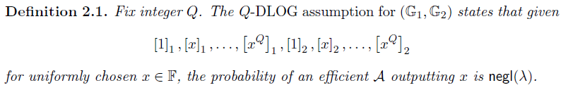
• 首先定义了类似[FKL18]中的Q-DLOG assumption：【即已知$[1{]}_1,[x{]}_1,\cdots ,[x^Q{]}_1,[1{]}_2,[x{]}_2,\cdots ,[x^Q{]}_2$，找到$x$的概率可忽略。】
  

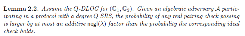
• 由Q-DLOG assumption，推出的lemma：【即real pairing check成立的概率与ideal check成立的概率相当。】
  

• Knowledge soundness in AGM 是指：
  Prover $P$ 和Verifier $V$之间的protocol $\mathcal{P}$ for relation $\mathcal{R}$ 具有Knowledge Soundness in the Algebraic Group Model的前提条件为——存在efficient $E$使得任意的algebraic adversary $\mathcal{A}$赢得如下游戏的概率可忽略：【又称 KS game】
  1）$\mathcal{A}$选择输入值$x$，并以Prover的角色运行$\mathcal{P}$ with input $x$；
  2）$E$可获取$A$在协议中的所有消息（包括linear combinations的系数），输出$w$；
  3）若同时满足以下情况，则$A$赢了：
  3.a）$V$在协议结束输出$acc$，即验证通过。且
  3.b）$(x,w)\notin \mathcal{R}$

3. [KZG10]的batch版本

本文协议的关键是实现了：
a batched version of the [KZG10] polynomial commitment scheme【与[MBKM19]中的附录C类似】，以满足 query multiple committed polynomials at multiple points。

接下来以有利于本文协议的方式来定义polynomial commitment schemes，特别地，其中的open流程对应的是a batched setting having multiple polynomials and evaluation points。

$d$-polynomial commitment scheme中包含如下算法：

• $gen(d)$——为随机算法，输出为SRS $srs$。
• $com(f,srs)$——输入为多项式$f\in {\mathbb{F}}_{<d}[X]$，输出为commitment $cm$ to $f$。
• $P_{PC}$和$V_{PC}$ 之间的public coin protocol $open$，针对的场景为：【具有completness和knowledge soundness in the algebraic group model属性。】
  – public info：SRS $srs$，$t=poly(\lambda )$，分别对应$f_1,\cdots ,f_t$的commitments $c{m}_1,\cdots ,c{m}_t$，evaluate points $z_1,\cdots ,z_t\in \mathbb{F}$ 以及 evaluation values $s_1,\cdots ,s_t\in \mathbb{F}$。
  – witness：多项式 $f_1,\cdots ,f_t\in {\mathbb{F}}_{<d}[X]$。
  – relations：$s_1=f_1(z_1),\cdots ,s_t=f_t(z_t)$ 且 $c{m}_1=com(f_1,srs),\cdots ,c{m}_t=com(f_t,srs)$。

3.1 batch open different polynomials at same points

根据[KZG10]和[MBKM19]，对以上$d$-polynomial commitment scheme实例化为：

• $gen(d)$——选择随机值$x\in \mathbb{F}$，输出SRS $srs=([1{]}_1,[x{]}_1,\cdots ,[x^{d-1}{]}_1,[1{]}_2,[x{]}_2)$。
• $com(f,srs):=[f(x){]}_1$。
• $P_{PC}$和$V_{PC}$ 之间的public coin protocol $open$，首先值考虑$z_1=\cdots =z_t=z$的情况， o p e n ( { c m i } , { z i } , { s i } ) open(\{cm_i\},\{z_i\},\{s_i\}) open({ cmi​},{ zi​},{ si​})的具体实现为：【即此处考虑的是：open diffierent polynomials at same points。】
  a）$V_{PC}$ 发送随机值$\gamma \in \mathbb{F}$。
  b）$P_{PC}$ 计算：
  $h(X):={\sum }_{i=1}^t{\gamma }^{i-1}\cdot \frac{f_i(X)-f_i(z)}{X-z}$
  并使用$srs$计算和发送 $W:=[h(x){]}_1$
  c）$V_{PC}$ 计算：
  $F:={\sum }_{i\in [t]}{\gamma }^i\cdot c{m}_i,v=[{\sum }_{i\in [t]}{\gamma }^i\cdot s_i{]}_1$
  d）当且仅当如下条件成立时，$V_{PC}$输出$acc$：
  $e(F-v,[1{]}_2)\cdot e(-W,[x-z{]}_2)=1$

需对以上实现进行knowledge soundness论证，即判断是否存在efficient $E$使得algebraic adversary $\mathcal{A}$取任意的$z=z_1=\cdots =z_t$赢得 KS game的概率可忽略。详细的分析思路为：【核心思想为Schwartz-Zippel Lemma】

3.2 batch open different polynomials at different points

当考虑：open diffierent polynomials at different points 时：

• 可将其看成是对open协议的并行执行，即每个open协议对应一个evaluation point和相应的polynomial evaluated at at that point；
• 然后引入generic method for batched randomized evaluation of pairing equations。

为了简化，本文将open协议中$z_1,\cdots ,z_t$分为两个不同的evaluation points（与本文主协议的实际情况对应）。将相应evaluation points表示为$z,z^{\prime }$，对应的polynomials数量分别为$t_1,t_2$，分别evaluate { f i } i ∈ [ t 1 ] \{f_i\}_{i\in [t_1]} { fi​}i∈[t1​]​ at $z$ 以及 evaluate { f i ′ } i ∈ [ t 2 ] \{f_i'\}_{i\in[t_2]} { fi′​}i∈[t2​]​ at $z^{\prime }$。

相应的open协议为—— o p e n ( { c m i } i ∈ [ t 1 ] , { c m i ′ } i ∈ [ t 2 ] , { z , z ′ } , { s i , s i ′ } ) open(\{cm_i\}_{i\in[t_1]},\{cm_i'\}_{i\in[t_2]},\{z,z'\},\{s_i,s_i'\}) open({ cmi​}i∈[t1​]​,{ cmi′​}i∈[t2​]​,{ z,z′},{ si​,si′​})：
a）$V_{PC}$ 发送随机值$\gamma ,{\gamma }^{\prime }\in \mathbb{F}$。
b）$P_{PC}$ 计算：
$h(X):={\sum }_{i=1}^{t_1}{\gamma }^{i-1}\cdot \frac{f_i(X)-f_i(z)}{X-z}$
$h^{\prime }(X):={\sum }_{i=1}^{t_2}{\gamma }^{\prime i-1}\cdot \frac{f_i^{\prime }(X)-f_i^{\prime }(z^{\prime })}{X-z^{\prime }}$
并使用$srs$计算和发送 $W:=[h(x){]}_1,W^{\prime }:=[h^{\prime }(x){]}_1$。
c）$V_{PC}$ 选择随机值$r^{\prime }\in \mathbb{F}$。
d）$V_{PC}$ 计算：
$F:=({\sum }_{i\in [t_1]}{\gamma }^{i-1}\cdot c{m}_i-[{\sum }_{i\in [t_1]}{\gamma }^{i-1}\cdot s_i{]}_1)+r^{\prime }\cdot ({\sum }_{i\in [t_2]}{\gamma }^{\prime i-1}\cdot c{m}_i^{\prime }-[{\sum }_{i\in [t_2]}{\gamma }^{\prime i-1}\cdot s_i^{\prime }{]}_1)$
当且仅当如下条件成立时，$V_{PC}$输出$acc$：
$e(F+z\cdot W+r^{\prime }{z}^{\prime }\cdot W^{\prime },[1{]}_2)\cdot e(-W-r^{\prime }\cdot W^{\prime },[x{]}_2)=1$

以上[KZG10] batch版本的算法效率分析如下：

• 对于$n\le d$且$f\in {\mathbb{F}}_{<n}[X]$时，计算$com(f)$需要$n$次${\mathbb{G}}_1$-exponentiations运算。
• 已知$\vec{z}:=(z_1,\cdots ,z_t)\in {\mathbb{F}}^t,f_1,\cdots ,f_t\in {\mathbb{F}}_{<d}[X]$，将$t^{\ast }$表示为$\vec{z}$中的distinct values数量；对于$i\in [t^{\ast }]$， d i : = m a x { d e g ( f i ) } i ∈ S i d_i:=max\{deg(f_i)\}_{i\in S_i} di​:=max{ deg(fi​)}i∈Si​​，其中$S_i$表示的是the set of indices $j$ such that $z_j$ equals the $i$'th distinct point in $\vec{z}$。令$c{m}_i=com(f_i)$，则 o p e n ( { c m i , f i , z i , s i } ) open(\{cm_i,f_i,z_i,s_i\}) open({ cmi​,fi​,zi​,si​}) 需要的计算量为：
  a）Prover需要${\sum }_{i\in [t^{\ast }]}{d}_i$次${\mathbb{G}}_1$-exponentiation运算。
  b）Verifier需要$t+2t^{\ast }-2$次${\mathbb{G}}_1$-exponentiation运算 和 2次pairing运算。

4. 理想化的low-degree protocols

对[KZG10]中的polynomial commitment scheme进行了抽象，形成的协议内容为：

• Prover将low-degree polynomials发送给可信第三方$\mathcal{I}$。
• Verifier可询问$\mathcal{I}$来确认Prover的这些多项式之间的关系，以及与Verifier提前知悉的预定义的多项式之间的关系。

形成的协议表示为$(d,D,t,l)$-polynomial protocol，其中$d,D,t,l$均为正整数。该协议在 Prover $P_{poly}$、Verifier $V_{poly}$ 以及 可信第三方 $\mathcal{I}$ 之间进行多轮执行，详细描述为：【具有completeness和Knowledge soundness属性。但实际实现时，不具有zero-knowledge 属性。具体见本论文中的Remark 4.4。】

• 1）协议定义中包含了一组预处理了的多项式$g_1,\cdots ,g_l\in {\mathbb{F}}_{<d}[X]$。
• 2）$P_{poly}$发送给$\mathcal{I}$的消息形式为：$f$ for $f\in {\mathbb{F}}_{<d}[X]$。若$P_{poly}$的消息不是这种形式，则协议终止。【注意此处不是$(f,n),n\le d$，具体原因见本论文中Remark 4.2。】
• 3）$P_{poly}$与$V_{poly}$之间的消息为任意形式的（但是本文将关注public coin protocols where the messages are simply random coins）。
• 4）在协议结束时，假设$f_1,\cdots ,f_t$为$P_{poly}$发送给$\mathcal{I}$的多项式。$V_{poly}$可询问$\mathcal{I}$ 是否 certain polynomial identities holds between { f 1 , ⋯   , f t , g 1 , ⋯   , g l } \{f_1,\cdots,f_t,g_1,\cdots,g_l\} { f1​,⋯,ft​,g1​,⋯,gl​}，其中identity的形式为：
  $F(X):=G(X,h_1(v_1(X)),\cdots ,h_M(v_M(X)))\equiv 0$
  其中 h i ∈ { f 1 , ⋯   , f t , g 1 , ⋯   , g l } , G ∈ F [ X , X 1 , ⋯   , X M ] , v 1 , ⋯   , v M ∈ F < d [ X ] h_i\in\{f_1,\cdots,f_t,g_1,\cdots,g_l\}, G\in\mathbb{F}[X,X_1,\cdots,X_M], v_1,\cdots,v_M\in\mathbb{F}_{<d}[X] hi​∈{ f1​,⋯,ft​,g1​,⋯,gl​},G∈F[X,X1​,⋯,XM​],v1​,⋯,vM​∈F<d​[X]，使得$F\in {\mathbb{F}}_{<D}[X]$ for every choice of $f_1,\cdots ,f_t$ made by $P_{poly}$ when following the protocol correctly。
• 5）当收到$\mathcal{I}$发送的关于identities的回复时，若所有identities均成立，则$V_{poly}$输出$acc$，否则输出$rej$。

4.1 polynomial protocols on range

实际要求$V_{poly}$ check if certain polynomial equations hold on a certain range of input values，而不仅是as a polynomial identity。
即，for subset $S\subset \mathbb{F}$，定义an $S$-ranged $(d,D,t,l)$-polynomial protocol identically to a $(d,D,t,l)$-polynomial protocol, except that the verifier asks if his identities hold on all points of $S$，rather than identically。（即该子集内的所有元素均符合相应特性）

只需额外再引入一个prover polynomial，就可将ranged protocol转换为polynomial protocol。相应有Lemma 4.5：
若$\mathcal{P}$为$S$-ranged $(d,D,t,l)$-polynomial protocol for $\mathcal{R}$，则可构建相应的 ( m a x { d , ∣ S ∣ , D − ∣ S ∣ } , D , t + 1 , l + 1 ) (max\{d,|S|,D-|S|\},D,t+1,l+1) (max{ d,∣S∣,D−∣S∣},D,t+1,l+1)-polynomial protocol ${\mathcal{P}}^{\ast }$ for $\mathcal{R}$。

在证明该Lemma之前，先了解Claim 4.6内容：


Lemma 4.5相应的证明为：

4.2 由polynomial protocols 到 protocols against algebraic adversaries

目的是：
可用第3节的polynomial commitment scheme来compile a polynomial protocol into one with knowledge soundness in the algebraic group model。

为了对以上转换的效率进行衡量，需定义相关技术来衡量$(d,D,t,l)$-polynomial protocol $\mathcal{P}$。

• 当$i\in [t]$，设置$d_i$为$\mathcal{P}$中由honest prover发送的$f_i$的最大degree，假设仅有一个identity $G(X,h_1(v_1(X)),\cdots ,h_M(v_M(X)))\equiv 0$ is checked by $V_{poly}$ in $\mathcal{P}$。
• 当$i\in [M]$时，设置$d_i^{\prime }$为the “matching” $d_j$。即若$h_i=f_j$有$d_i^{\prime }=d_j$；若$h_i=g_j$有$d_i^{\prime }=deg(g_j)$。
• 设 $t^{\ast }=t^{\ast }(\mathcal{P})$ 为$v_1,\cdots ,v_M$ 中的不同多项式的数量。设$S_1\cup \cdots \cup S_{t^{\ast }}=[M]$为相应的 partition of $[M]$ 。当$j\in [t^{\ast }]$，令 e j : = m a x { d i ′ } i ∈ S j e_j:=max\{d_i'\}_{i\in S_j} ej​:=max{ di′​}i∈Sj​​。
• 最后，定义$e(\mathcal{P}):={\sum }_{i\in [t]}(d_i+1)+{\sum }_{j\in [t^{\ast }]}{e}_j$

Lemma 4.7 内容为：【详细的证明可参见论文P17~P18。】
若$\mathcal{P}$为$(d,D,t,l)$-polynomial protocol for $\mathcal{R}$，其中仅有一个identity is checked by $V_{poly}$，则可构建相应的protocol ${\mathcal{P}}^{\ast }$ for $\mathcal{R}$ with knowledge soundness in the Algebraic Group Model under $2d$-DLOG 具有如下属性：

• 1）${\mathcal{P}}^{\ast }$中的Prover需要 $e(\mathcal{P})$次${\mathbb{G}}_1$-exponentiation 运算。
• 2）总的communication cost为 $t+t^{\ast }(\mathcal{P})$个${\mathbb{G}}_1$ elements 和 $M$ 个 $\mathbb{F}$-elements。【可借助Mary Maller优化，进一步reduce $\mathbb{F}$-elements 的数量。】
• 3）Verifier需要 $t+t^{\ast }(\mathcal{P})$ 次 ${\mathbb{G}}_1$-exponentiations运算，2次pairing运算和1次evaluation of $G$。

4.2.1 优化 $\mathbb{F}$-elements 数量

借助Mary Maller优化，进一步reduce $\mathbb{F}$-elements 的数量：
假设$V$想要check identity $h_1(X)h_2(X)-h_3(X)\equiv 0$，之前的方法是$P$ 发送values of $h_1,h_2,h_3$ at random $x\in \mathbb{F}$，然后$V$验证$h_1(x)h_2(x)-h_3(x)=0$是否成立。整个过程中$P$发送了3个field elements。
现在，可让$P$仅发送$c:=h_1(x)$，然后运行open protocol来验证多项式 $L(X):=x\cdot h_2(X)-h_3(X)$是否为zero at $x$。【同时注意，可计算$com(L)=c\cdot com(h_2)-com(h_3)$。】

因此，需定义另一种技术手段来衡量a polynomial protocol。
为了简化，再次假设$V_{poly}$仅需验证one identity $F$。现定义$r(\mathcal{P})$为the minimal size of a subset $S\subset [M]$，满足：

• $([M]\setminus S)\subset S_i$ for one of the subsets $S_i$ of the partition descrbed before Lemma 4.7。
• polynomial $G$：
  $F(X):=G(X,h_1(v_1(X)),\cdots ,h_M(v_M(X)))$
  具有degree zero or one as a polynomial in the variables { X j } j ∈ [ M ] ∖ S \{X_j\}_{j\in[M]\setminus S} { Xj​}j∈[M]∖S​ whose coefficients are polynomials in $X$ and { X j } j ∈ S \{X_j\}_{j\in S} { Xj​}j∈S​。

假设有$r:=r(\mathcal{P})<M$，可对Lemma 4.7做如下reduction，使得Prover发送的$\mathbb{F}$-elements数量由$M$降为$r$个：

5. Polynomial protocols for identifying permutations

本文universal SNARK的核心为 ”permutation check“，受[BG12]中的permutation argument 和 [BCC+16][MBKM19]的变种 启发。

相比于[MBKM19]，本文算法的由于采用的是单变量多项式和multiplicative subgroups，实现的协议更简单。

要求$n\le d$，其中$n$为the degree of the honest prover’s polynomials，$d$为the bound we actually enforce on malicous provers。
相应地，在分析prover efficiency和描述”official“ protocol input时，可将degree bound 看成为$n$，而分析soundness时，可假设degree bound 为$d$。

当$i\in [n]$时，$L_i(X)$ 表示 the element of ${\mathbb{F}}_{<n}[X]$ with $L_i({\mathbf{g}}^i)=1$ and $L_i(a)=0$ for $a\in H$ different from ${\mathbf{g}}^i$，即 { L i } i ∈ [ n ] \{L_i\}_{i\in [n]} { Li​}i∈[n]​为a Lagrange basis for H。
同时注意，$L_i$可”reduce point checks to range checks“。

Claim 5.1内容为：
若$i\in [n],Z,Z^{\ast }\in \mathbb{F}[X]$，则当且仅当$Z({\mathbf{g}}^i)=Z^{\ast }({\mathbf{g}}^i)$时，有$L_i(a)(Z(a)-Z^{\ast }(a))=0$ for each $a\in H$。

当$f,g\in {\mathbb{F}}_{<d}[X]$和permutation $\sigma :[n]\to [n]$时，若对于每一个$a\in H$，都有$g({\mathbf{g}}^i)=f({\mathbf{g}}^{\sigma (i)})$，则可表示为：$g=\sigma (f)$。

5.1 证明$g=\sigma (f)$的ranged polynomial protocol

接下来将构建a ranged polynomial protocol来证明$g=\sigma (f)$。
针对的场景为：

• preprocessed polynomials：有polynomial $S_{ID}\in {\mathbb{F}}_{<n}[X]$ defined by $S_{ID}({\mathbf{g}}^i)=i$ for each $i\in [n]$，以及polynomial $S_{\sigma }\in {\mathbb{F}}_{<n}[X]$ defined by $S_{\sigma }({\mathbf{g}}^i)=\sigma (i)$ for each $i\in [n]$。【注意，有${\mathbf{g}}^{n+1}=\mathbf{g}$。】

• inputs 输入为：$f,g\in {\mathbb{F}}_{<n}[X]$。

• Protocol 具体协议实现为：
  1）$V_{poly}$ 发送随机值 $\beta ,\gamma \in \mathbb{F}$ 给 $P_{poly}$。
  2）令 $f^{\prime }:=f+\beta \cdot S_{ID}+\gamma ,g^{\prime }=g+beta\cdot S_{\sigma }+\gamma$，则对 $i\in [n]$有：
  $f^{\prime }({\mathbf{g}}^i)=f({\mathbf{g}}^i)+\beta \cdot i+\gamma ,g^{\prime }({\mathbf{g}}^i)=g({\mathbf{g}}^i)+\beta \cdot \sigma (i)+\gamma$
  3）$P_{poly}$ 计算$Z\in {\mathbb{F}}_{<n}[X]$，使得$Z(\mathbf{g})=1$；且对于 i ∈ { 2 , ⋯   , n } i\in\{2,\cdots,n\} i∈{ 2,⋯,n}，有：
  $Z({\mathbf{g}}^i)={\prod }_{1\le j<i}{f}^{\prime }({\mathbf{g}}^j)/g^{\prime }({\mathbf{g}}^j)$
  （one of the product elements为undefined的概率可忽略。）
  4）$P_{poly}$将$Z$发送给$\mathcal{I}$。
  5）$V_{poly}$对所有的$a\in H$，当且仅当如下两个条件都成立时输出$acc$：
  5.a）$L_1(a)(Z(a)-1)=0$【即满足$Z(\mathbf{g})=1$】
  5.b）$Z(a)f^{\prime }(a)=g^{\prime }(a)Z(a\cdot \mathbf{g})$ 【即满足$Z({\mathbf{g}}^i)={\prod }_{1\le j<i}{f}^{\prime }({\mathbf{g}}^j)/g^{\prime }({\mathbf{g}}^j)$】

5.2 checking “extended” permutations

本文的目的是：
check a permutation “across” the values of several polynomials。

假设有多个多项式 $f_1,\cdots ,f_k\in {\mathbb{F}}_{<d}[X]$ 和 permutation $\sigma :[kn]\to [kn]$。

对于$(g_1,\cdots ,g_k)\in ({\mathbb{F}}_{<d}[X]{)}^k$，当以下条件成立时，可称 $(g_1,\cdots ,g_k)=\sigma (f_1,\cdots ,f_k)$：
定义序列 $(f_{(1)},\cdots ,f_{(kn)}),(g_{(1)},\cdots ,g_{(kn)})\in {\mathbb{F}}^{kn}$ 为：
$f_{((j-1)\cdot n+i)}:=f_j({\mathbf{g}}^i),g_{((j-1)\cdot n+i)}:=g_j({\mathbf{g}}^i)$
for each $j\in [k],i\in [n]$。则有$g_l=f_{\sigma (l)}$ for each $l\in [kn]$。

针对的场景为：

• Preprocessed polynomials有：
  $S_{I{D}_1},\cdots ,S_{I{D}_k}\in {\mathbb{F}}_{<n}[X]$ defined by $S_{I{D}_j}({\mathbf{g}}^i)=(j-1)\cdot n+i$ for each $i\in [n]$ 【实际上仅需要$S_{ID}=S_{I{D}_1}$就足够了，其它的$S_{I{D}_j}(x)$均可计算出来——$S_{I{D}_j}(x)=S_{ID}(x)+(j-1)\cdot n$】
  对于每一个的$j\in [k]$，有$S_{{\sigma }_j}\in {\mathbb{F}}_{<n}[X]$ defined by $S_{{\sigma }_j}({\mathbf{g}}^i)=\sigma ((j-1)\cdot n+i)$ for each $i\in [n]$。

• inputs 输入为：$f_1,\cdots ,f_k,g_1,\cdots ,g_k\in {\mathbb{F}}_{<n}[X]$。

• Protocol 相应的协议实现为：
  1）$V_{poly}$ 发送随机值 $\beta ,\gamma \in \mathbb{F}$ 给 $P_{poly}$。
  2）令 $f_j^{\prime }:=f_j+\beta \cdot S_{I{D}_j}+\gamma ,g_j^{\prime }=g_j+beta\cdot S_{{\sigma }_j}+\gamma$，则对 $j\in [k],i\in [n]$有：
  $f_j^{\prime }({\mathbf{g}}^i)=f_j({\mathbf{g}}^i)+\beta \cdot ((j-1)\cdot n+i)+\gamma ,g_j^{\prime }({\mathbf{g}}^i)=g_j({\mathbf{g}}^i)+\beta \cdot \sigma ((j-1)\cdot n+i)+\gamma$
  3）定义$f^{\prime },g^{\prime }\in {\mathbb{F}}_{<kn}[X]$为：
  $f^{\prime }(X):={\prod }_{j\in [k]}{f}_j^{\prime }(X),g^{\prime }(X):={\prod }_{j\in [k]}{g}_j^{\prime }(X)$
  4）$P_{poly}$ 计算$Z\in {\mathbb{F}}_{<n}[X]$，使得$Z(\mathbf{g})=1$；且对于 i ∈ { 2 , ⋯   , n } i\in\{2,\cdots,n\} i∈{ 2,⋯,n}，有：
  $Z({\mathbf{g}}^i)={\prod }_{1\le j<i}{f}^{\prime }({\mathbf{g}}^j)/g^{\prime }({\mathbf{g}}^j)$
  （one of the product elements为undefined的概率可忽略。）
  5）$P_{poly}$将$Z$发送给$\mathcal{I}$。
  6）$V_{poly}$对所有的$a\in H$，当且仅当如下两个条件都成立时输出$acc$：
  6.a）$L_1(a)(Z(a)-1)=0$【即满足$Z(\mathbf{g})=1$】
  6.b）$Z(a)f^{\prime }(a)=g^{\prime }(a)Z(a\cdot \mathbf{g})$ 【即满足$Z({\mathbf{g}}^i)={\prod }_{1\le j<i}{f}^{\prime }({\mathbf{g}}^j)/g^{\prime }({\mathbf{g}}^j)$】

5.3 checking “extended copy constraints” using a permutation

最终本文主协议中实际的primitive为：
令 T = { T 1 , ⋯   , T s } \mathcal{T}=\{T_1,\cdots,T_s\} T={ T1​,⋯,Ts​} 为 a partition of $[kn]$ into disjoint blocks。

对于特定的$f_1,\cdots ,f_k\in {\mathbb{F}}_{<n}[X]$，定义$(f_{(1)},\cdots ,f_{(kn)})\in {\mathbb{F}}^{kn}$，若有$f_{(l)}=f_{(l^{\prime })}$ whenever $l,l^{\prime }$ belong to the same block of $\mathcal{T}$，则可称 $f_1,\cdots ,f_k$ copy-satisfy $\mathcal{T}$。

5.2节的protocol for extended permutations可直接拿来check whether $f_1,\cdots ,f_k$ satisfy $\mathcal{T}$，具体为：
定义a permutation $\sigma (\mathcal{T})$ on $[kn]$，使得对于$\mathcal{T}$中的每一个block $T_i$，$\sigma (\mathcal{T})$ 包含了a cycle going over all elements of $T_i$。
则 当且仅当$(f_1,\cdots ,f_k)=\sigma (f_1,\cdots ,f_k)$，有 $(f_1,\cdots ,f_k)$ copy-satisfy $\mathcal{T}$。

6. Constraint systems

有$n\le m\le 2n$。
将fan-in two arithmetic circuits of unlimited fan-out with $n$ gates and $m$ wires 以constraint system的形式来表达。

constraint system $\mathcal{L}=(\mathcal{V},\mathcal{Q})$定义如下：

• $\mathcal{V}$ 的形式为：$\mathcal{V}=(\vec{a},\vec{b},\vec{c})$，其中$\vec{a},\vec{b},\vec{c}\in [m{]}^n$，可将$\vec{a},\vec{b},\vec{c}$ 看成是 $\mathcal{L}$的左侧、右侧和输出序列。
• $\mathcal{Q}$ 的形式为：$\mathcal{Q}=({\vec{q}}_L,{\vec{q}}_R,{\vec{q}}_O,{\vec{q}}_M,{\vec{q}}_C)\in ({\mathbb{F}}^n{)}^5$，其中${\vec{q}}_L,{\vec{q}}_R,{\vec{q}}_O,{\vec{q}}_M,{\vec{q}}_C\in {\mathbb{F}}^n$ 可看成是”selector vectors“。

称$\vec{x}\in {\mathbb{F}}^m$ satisfies $\mathcal{L}$ 当且仅当 对于每一个$i\in [n]$ 均有：
$({\vec{q}}_L{)}_i\cdot {\vec{x}}_{{\vec{a}}_i}+({\vec{q}}_R{)}_i\cdot {\vec{x}}_{{\vec{b}}_i}+({\vec{q}}_O{)}_i\cdot {\vec{x}}_{{\vec{c}}_i}+({\vec{q}}_M{)}_i\cdot ({\vec{x}}_{{\vec{a}}_i}\cdot {\vec{x}}_{{\vec{b}}_i})+({\vec{q}}_C{)}_i=0$

定义正整数$l\le m$，子集$\mathcal{I}\subset [m]$ of “public inputs”。
进一步不失一般性地假设 I = { 1 , ⋯   , l } \mathcal{I}=\{1,\cdots,l\} I={ 1,⋯,l}。
定义relation ${\mathcal{R}}_{\mathcal{L}}$为：
the set of pairs $(\vec{x},\vec{w})$ with $\vec{x}\in {\mathbb{F}}^l,w\in {\mathbb{F}}^{m-l}$，使得$\mathbf{x}:=(\vec{x},\vec{w})$ satisfies $\mathcal{L}$。

则相应的constraint system实例化分类有：

• Arithmetic circuits
• Booleanity constraints
• public inputs constraints

6.1 arithmetic circuits 对应的constraint systems

针对的是：fan-in 2 circuit of $n$ gates，gate类型仅支持加法或乘法，其constraint可表示为：

• 1）$m$用于表示线的数量，每根线对应一个index $i\in [m]$。

对于每一个门，$i\in [n]$，有：

• 2）依次设置$a_i,b_i,c_i$为第$i$个门的left/right/output wire index。
• 3）当第$i$个门为乘法门时，依次设置$({\vec{q}}_L{)}_i=0,({\vec{q}}_R{)}_i=0,({\vec{q}}_M{)}_i=1,({\vec{q}}_O{)}_i=-1$。
• 4）当第$i$个门为加法门时，依次设置$({\vec{q}}_L{)}_i=1,({\vec{q}}_R{)}_i=1,({\vec{q}}_M{)}_i=0,({\vec{q}}_O{)}_i=-1$。【注意，可设置$({\vec{q}}_L{)}_i,({\vec{q}}_R{)}_i$为非零值来表达“linear combination gates”。】
• 5）总是设置$({\vec{q}}_C{)}_i=0$。

6.2 booleanity constraints

针对要求 x j ∈ { 0 , 1 } \mathbf{x}_j\in\{0,1\} xj​∈{ 0,1} for some $j\in [m]$的场景。
对于每一个门，$i\in [n]$，有：
$a_i=b_i=j,({\vec{q}}_L{)}_i=-1,({\vec{q}}_M{)}_i=1,({\vec{q}}_R{)}_i=({\vec{q}}_O{)}_i=({\vec{q}}_C{)}_i=0$

6.4 public inputs constraints

针对public inputs ${\mathbf{x}}_1,\cdots ,{\mathbf{x}}_l$ 的约束，即要求对于某个门$i\in [n]$，满足${\mathbf{x}}_j=x_j$，有：
$a_i=j,({\vec{q}}_L{)}_i=1,({\vec{q}}_M{)}_i=({\vec{q}}_R{)}_i=({\vec{q}}_O{)}_i=0,({\vec{q}}_C{)}_i=-x_j$

7. 主协议

令 $\mathcal{L}=(\mathcal{V},\mathcal{Q})$ 为第6节对应的constraint system，对应的relation为${\mathcal{R}}_{\mathcal{L}}$。

partition of $\mathcal{L}$ 表示为${\mathcal{T}}_{\mathcal{L}}$。

假设：$\mathcal{V}=(\vec{a},\vec{b},\vec{c})$，可将其看成是a vector $\vec{V}$ in $[m{]}^{3n}$。
对于$i\in [m]$，令$T_i\subset [3n]$为the set of indices $j\in [3n]$，使得$\vec{V}=i$，则可定义：
T L : = { T i } i ∈ [ m ] \mathcal{T}_{\mathscr{L}}:=\{T_i\}_{i\in[m]} TL​:={ Ti​}i∈[m]​

for $i\in [l]$，当满足如下条件时，可称$\mathcal{L}$ is prepared for $l$ public inputs：
$a_i=i,({\vec{q}}_L{)}_i=1,({\vec{q}}_M{)}_i=({\vec{q}}_R{)}_i=({\vec{q}}_O{)}_i=0,({\vec{q}}_C{)}_i=0$

记住 H = { g , ⋯   , g n } H=\{\mathbf{g},\cdots,\mathbf{g}^n\} H={ g,⋯,gn}，为${\mathcal{R}}_{\mathcal{L}}$构建的$H$-ranged polynomial protocol为：

• Preprocessing：
  令$\sigma =\sigma ({\mathcal{T}}_{\mathcal{L}})$。
  具体$S_{I{D}_1},S_{I{D}_2},S_{I{D}_3},S_{{\sigma }_1},S_{{\sigma }_2},S_{{\sigma }_3}\in {\mathbb{F}}_{<n}[X]$多项式的定义可参见 5.1节“checking “extended” permutations”。
  对于每个门$i\in [n]$，相应的多项式$q_L,q_R,q_O,q_M,q_C\in {\mathbb{F}}_{<n}[X]$的定义为：
  $q_L({\mathbf{g}}^i):=({\vec{q}}_L{)}_i,q_R({\mathbf{g}}^i):=({\vec{q}}_R{)}_i,q_O({\mathbf{g}}^i):=({\vec{q}}_O{)}_i,q_M({\mathbf{g}}^i):=({\vec{q}}_M{)}_i,q_C({\mathbf{g}}^i):=({\vec{q}}_C{)}_i$

• 具体的协议实现为：【$H$-ranged polynomial protocol for relation ${\mathcal{R}}_{\mathcal{L}}$。】
  1）令$\mathbf{x}\in {\mathbb{F}}^m$为$P_{poly}$的assignment，其与public input $\vec{x}$保持一致性。$P_{poly}$输出了3个多项式$f_L,f_R,f_O\in {\mathbb{F}}_{<n}[X]$，使得对每一个门$i\in [n]$，有：
  $f_L(i)={\mathbf{x}}_{a_i},f_R(i)={\mathbf{x}}_{b_i},f_O(i)={\mathbf{x}}_{c_i}$
  $P_{poly}$将$f_L,f_R,f_O$发送给$\mathcal{I}$。
  2）$P_{poly}$和$V_{poly}$都运行 the extended permutation check 协议，使用the permutation $\sigma$ between $(f_L,f_R,f_O)$ and itself。
  如 5.3节“checking “extended copy constraints” using a permutation” 所解释的，其exactly checks whether $(f_L,f_R,f_O)$ copy-satisfies ${\mathcal{T}}_{\mathcal{L}}$。
  3）$V_{poly}$ 计算“Public input polynomial”：
  $PI(X):={\sum }_{i\in [l]}-x_i\cdot L_i(X)$
  4）$V_{poly}$ 基于$H$以下identity是否成立：
  $q_L\cdot f_L+q_R\cdot f_R+q_O\cdot f_O+q_M\cdot f_L\cdot f_R+(q_C+PI)=0$

以上协议对应的计算量和communication cost为：

• Prover 需要$11n+2$次${\mathbb{G}}_1$-exponentiations运算；【$e(\mathcal{P})=11n+2$，因其中有$7n+1$ cost of commitments，the maximal degree among the polynomial evaluated at $x$为$3n$ 以及 the maximum degree among polynomials evaluated at $x/\mathbf{g}$ 为 $n+1$。】
• 总的communication cost为 7个${\mathbb{G}}_1$-elements和8个$\mathbb{F}$-elements。
• $t^{\ast }\mathcal{P}=2$，因有2个distinct evaluation points。
• $r(\mathcal{P})\le 8$。

8. 最终完整的协议

为了便于读者理解，整理了 the full final protocol。

在此之前，都未考虑zero-knowledge属性，而此时，将通过增加 random multiples of $Z_H$ to the witness based-polynomials 来实现zero-knowledge属性。这种方式不会影响satisfiability，但可create a situation where the values are either completely uniform or determined by verifier equations。【实际上，为实现优化的FFT性能，一般要求$H$为a multiplicative group with few points omitted so that the degrees even after adding these random multiples are smaller than the group order $n$。这将要求a slight complication of the grand product argument with separate constraints for $Z$ staring and ending at one，as our actual set $H$ does not “wrap” anymore。】

明确定义multiplicative group $H$包含了$n$’th roots of unity in ${\mathbb{F}}_p$，其中$\omega$ 为 a primitive $n$'th root of unity and a generator of $H$，即 H = { 1 , ω , ⋯   , ω n − 1 } H=\{1,\omega,\cdots,\omega^{n-1}\} H={ 1,ω,⋯,ωn−1}。

假设circuit中的门数量不超过$n$。

同时，本文还包含了来自Vitalik的优化建议——定义the identity permutations through degree-1 polynomials。这种identity permutations必须map 每一个wire value TO a unique element $\in \mathbb{F}$。可通过定义$S_{I{D}_1}(X)=X,S_{I{D}_2}(X)=k_{1}X,S_{I{D}_3}(X)=k_{2}X$来实现，其中$k_1,k_2$为quadratic non-residues $\in \mathbb{F}$。这可effectively map 每一个wire value TO a root of unity in $H$，其中right wires和ouput wires分别具有额外的mulitplicative factor of $k_1,k_2$。通过所实现的identity permutation via degree-1 polynomials，其evaluations可由Verifier来直接计算。这将减少proof size中的1个$\mathbb{F}$ element的同时，还可以减少Prover运行FFT的次数 以及 减少Verifier 的1个scalar multiplication计算。

8.1 用于定义特定circuit的多项式

以下这些多项式，与integer $n$一起，唯一定义了a universal SNARK circuit：

• $q_M(X),q_L(X),q_R(X),q_O(X),q_C(X)$ 为“selector”多项式，定义了circuit’s arithmetisation。
• $S_{I{D}_1}(X)=X,S_{I{D}_2}(X)=k_{1}X,S_{I{D}_3}(X)=k_{2}X$ 为 用于$\mathbf{a},\mathbf{b},\mathbf{c}$的identity permutation。其中$k_1,k_2\in \mathbb{F}$ 满足 $H,k_1\cdot H,k_2\cdot H$为distinct cosets of $H$ in ${\mathbb{F}}^{\ast }$，即包含有$3n$个不同的元素。（如，当$\omega$为quadratic residue in $\mathbb{F}$时，取$k_1$为任意quadratic non-residue，取$k_2$为a quadratic non-residue not contained in $k_1\cdot H$。）
• $S_{{\sigma }_1}(X),S_{{\sigma }_2}(X),S_{{\sigma }_3}(X)$ 为 用于$\mathbf{a},\mathbf{b},\mathbf{c}$的copy permutation。
• $n$为特定circuit中总的门数量。由$V$用于计算vanishing polynomial：
  $Z_H(X)=X^n-1$

8.2 对wire values 的commitments

proof的witness实际为the wire value witnesses $(w_i{)}_{i=1}^{3n}$。
Kate polynomial commitments具有computationally binding属性，对wire value witnesses的commItment可表示为$[a{]}_1,[b{]}_1,[c{]}_1$，其会用到包含 group elements $(x\cdot [1{]}_1,\cdots ,x^n\cdot [1{]}_1)$ 的structured reference string。

8.3 un-rolled universal SNARK proof relation表示

完整的un-rolled universal SNARK proof relation表示为：
R s n a r k ( λ ) = { ( x , w , c r s ) = ( ( w i ) i ∈ [ l ] ) , ( ( w i ) i = 1 , i ∉ [ l ] 3 n ) , ( ( q M i , q L i , q R i , q O i , q C i ) i = 1 n , n , σ ( x ) ) For all  i ∈ { 1 , ⋯   , 3 n } : w i ∈ F p ,  and for all  i ∈ { 1 , ⋯   , n } : w i w n + i q M i + w i q L i + w n + i q R i + w 2 n + i q O i + q C i = 0  and for all  i ∈ { 1 , ⋯   , 3 n } : w i = w σ ( i ) } \mathcal{R}_{snark}(\lambda)=\begin{Bmatrix} (x,w,crs)=((w_i)_{i\in[l]}),((w_i)_{i=1,i\notin[l]}^{3n}),\\ ((q_{M_i},q_{L_i},q_{R_i},q_{O_i},q_{C_i})_{i=1}^n,n,\sigma(x))\\ \text{For all } i\in\{1,\cdots,3n\}: w_i\in\mathbb{F}_p, \text{ and for all } i\in\{1,\cdots,n\}:\\ w_iw_{n+i}q_{M_i}+w_iq_{L_i}+w_{n+i}q_{R_i}+w_{2n+i}q_{O_i}+q_{C_i}=0\\ \text{ and for all } i\in\{1,\cdots,3n\}: w_i=w_{\sigma(i)} \end{Bmatrix} Rsnark​(λ)=⎩⎪⎪⎪⎪⎨⎪⎪⎪⎪⎧​(x,w,crs)=((wi​)i∈[l]​),((wi​)i=1,i∈/​[l]3n​),((qMi​​,qLi​​,qRi​​,qOi​​,qCi​​)i=1n​,n,σ(x))For all i∈{ 1,⋯,3n}:wi​∈Fp​, and for all i∈{ 1,⋯,n}:wi​wn+i​qMi​​+wi​qLi​​+wn+i​qRi​​+w2n+i​qOi​​+qCi​​=0 and for all i∈{ 1,⋯,3n}:wi​=wσ(i)​​⎭⎪⎪⎪⎪⎬⎪⎪⎪⎪⎫​

8.4 具体协议实现

本文使用Fiat-Shamir heuristic来实现non-interactive protocol。
使用transcript来表示：
the concatenation of the common preprocessed input, and public input, and the proof elements written by the prover up to a certain point in time。

本文使用transcript来获取random challenges via Fiat-Shamir。

可将以下写“compute challenges”的部分替换为：Verifier 发送random field elements来改为interactive protocol。

使用$\mathcal{R}$ 来表示hash函数， R : { 0 , 1 } ∗ → F p \mathcal{R}:\{0,1\}^*\rightarrow\mathbb{F}_p R:{ 0,1}∗→Fp​ 来模拟the random oracle。

• Common preprocessed input有：
  $n,(x\cdot [1{]}_1,\cdots ,x^{n+5}\cdot [1{]}_1),(q_{M_i},q_{L_i},q_{R_i},q_{O_i},q_{C_i}{)}_{i=1}^n,\sigma (X)$
  $q_M(X)={\sum }_{i=1}^n{q}_{M_i}{L}_i(X),$
  $q_L(X)={\sum }_{i=1}^n{q}_{L_i}{L}_i(X),$
  $q_R(X)={\sum }_{i=1}^n{q}_{R_i}{L}_i(X),$
  $q_O(X)={\sum }_{i=1}^n{q}_{O_i}{L}_i(X),$
  $q_C(X)={\sum }_{i=1}^n{q}_{C_i}{L}_i(X),$
  $S_{{\sigma }_1}(X)={\sum }_{i=1}^n\sigma (i)L_i(X),$
  $S_{{\sigma }_2}(X)={\sum }_{i=1}^n\sigma (n+i)L_i(X),$
  $S_{{\sigma }_3}(X)={\sum }_{i=1}^n\sigma (2n+i)L_i(X)$

• Public input有：
  $l,(w_i{)}_{i\in [l]}$

8.4.1 Prover $P$ 端算法

Prover input 有：$(w_i{)}_{i\in [3n]}$

• Round 1 第一轮：
  1）生成随机blinding scalars $(b_1,\cdots ,b_9)\in {\mathbb{F}}_p$
  2）计算wire 多项式 $a(X),b(X),c(X)$：
  $a(X)=(b_{1}X+b_2)Z_H(X)+{\sum }_{i=1}^n{w}_i{L}_i(X)$
  $b(X)=(b_{3}X+b_4)Z_H(X)+{\sum }_{i=1}^n{w}_{n+i}{L}_i(X)$
  $c(X)=(b_{5}X+b_6)Z_H(X)+{\sum }_{i=1}^n{w}_{2n+i}{L}_i(X)$
  3）计算：$[a{]}_1:=[a(x){]}_1,[b{]}_1:=[b(x){]}_1,[c{]}_1:=[c(x){]}_1$
  第一轮$P$的输出为$([a{]}_1,[b{]}_1,[c{]}_1)$。

• Round 2 第二轮：
  1）计算permutation challeges $(\beta ,\gamma )\in {\mathbb{F}}_p$：
  $\beta =\mathcal{R}(transcript,0),\gamma =\mathcal{R}(transcript,1)$
  2）计算permutation polynomial $z(X)$：
  $z(X)=(b_7{X}^2+b_{8}X+b_9)Z_H(X)+L_1(X)+{\sum }_{i=1}^{n-1}(L_{i+1}(X){\prod }_{j=1}^i\frac{(w_j+\beta {\omega }^{j-1}+\gamma )(w_{n+j}+\beta k_1{\omega }^{j-1}+\gamma )(w_{2n+j}+\beta k_2{\omega }^{j-1}+\gamma )}{(w_j+\sigma (j)\beta +\gamma )(w_{n+j}+\sigma (n+j)\beta +\gamma )(w_{2n+j}+\sigma (2n+j)\beta +\gamma )})$
  3）计算：$[z{]}_1:=[z(x){]}_1$
  第二轮$P$的输出为$([z{]}_1)$。

• Round 3 第三轮：
  1）计算quotient challenege $\alpha \in {\mathbb{F}}_p$：
  $\alpha =\mathcal{R}(transcript)$
  2）计算quotient polynomial $t(X)$：
  $t(X)=(a(X)b(X)q_M(X)+a(X)q_L(X)+b(X)q_R(X)+c(X)q_O(X)+PI(X)+q_C(X))\frac{1}{Z_H(X)}+((a(X)+\beta X+\gamma )(b(X)+\beta k_{1}X+\gamma )(c(X)+\beta k_{2}X+\gamma )z(X))\frac{\alpha }{Z_H(X)}-((a(X)+\beta S_{{\sigma }_1}(X)+\gamma )(b(X)+\beta S_{{\sigma }_2}(X)+\gamma )(c(X)+\beta S_{{\sigma }_3}(X)+\gamma )z(X\omega ))\frac{\alpha }{Z_H(X)}+(z(X)-1)L_1(X)\frac{{\alpha }^2}{Z_H(X)}$
  将$t(X)$拆分为degree $<n$ 多项式$t_{lo}(X),t_{mid}(X)$ 和 degree $\le n+5$ 多项式$t_{hi}(X)$表示为：
  $t(X)=t_{lo}(X)+X^n{t}_{mid}(X)+X^{2n}{t}_{hi}(X)$
  3）计算：$[t_{lo}{]}_1:=[t_{lo}(x){]}_1,[t_{mid}{]}_1:=[t_{mid}(x){]}_1,[t_{hi}{]}_1:=[t_{hi}(x){]}_1$
  第三轮$P$的输出为$([t_{lo}{]}_1,[t_{mid}{]}_1,[t_{hi}{]}_1)$。

• Round 4 第四轮：
  1）计算evaluation challenge $\vartheta \in {\mathbb{F}}_p$：
  $\vartheta =\mathcal{R}(transcript)$
  2）计算opening evaluations：
  $\bar{a}=a(\vartheta ),\bar{b}=b(\vartheta ),\bar{c}=c(\vartheta ),{\bar{s}}_{{\sigma }_1}=S_{{\sigma }_1}(\vartheta ),{\bar{s}}_{{\sigma }_2}=S_{{\sigma }_2}(\vartheta ),\bar{t}=t(\vartheta ),{\bar{z}}_{\omega }=t(\vartheta \omega )$
  3）计算linearisation polynomial $r(X)$：
  $r(X)=(\bar{a}\bar{b}\cdot q_M(X)+\bar{a}\cdot q_L(X)+\bar{b}\cdot q_R(X)+\bar{c}\cdot q_O(X)+q_C(X))+((\bar{a}+\beta \vartheta +\gamma )(\bar{b}+\beta k_1\vartheta +\gamma )(\bar{c}+\beta k_2\vartheta +\gamma )\cdot z(X))\alpha -((\bar{a}+\beta {\bar{s}}_{{\sigma }_1}+\gamma )(\bar{b}+\beta {\bar{s}}_{{\sigma }_2}+\gamma )\beta {\bar{z}}_{\omega }\cdot S_{{\sigma }_3}(X))\alpha +(z(X))L_1(\vartheta ){\alpha }^2$
  4）计算 linearsation evaluation $\bar{r}=r(\vartheta )$
  第四轮$P$的输出为$(\bar{a},\bar{b},\bar{c},{\bar{s}}_{{\sigma }_1},{\bar{s}}_{{\sigma }_2},{\bar{z}}_{\omega },\bar{t},\bar{r})$。

• Round 5 第五轮：
  1）计算opening challenge $v\in {\mathbb{F}}_p$：
  $v=\mathcal{R}(transcript)$
  2）计算opening proof polynomial $W_{\vartheta }(X)$：
  $W_{\vartheta }(X)=\frac{1}{X-\vartheta }((t_{lo}(X)+{\vartheta }^n{t}_{mid}(X)+{\vartheta }^{2n}{t}_{hi}(X)-\bar{t})+v(r(X)-\bar{r})+v^2(a(X)-\bar{a})+v^3(b(X)-\bar{b})+v^4(c(X)-\bar{c})+v^5(S_{{\sigma }_1}(X)-{\bar{s}}_{{\sigma }_1})+v^6(S_{{\sigma }_2}(X)-{\bar{s}}_{{\sigma }_2}))$
  3）计算opening proof plynomial $W_{\vartheta \omega }(X)$：
  $W_{\vartheta \omega }(X)=\frac{(z(X)-{\bar{z}}_{\omega })}{X-\vartheta \omega }$
  4）计算 $[W_{\vartheta }{]}_1:=[W_{\vartheta }(x){]}_1,[W_{\vartheta \omega }{]}_1:=[W_{\vartheta \omega }(x){]}_1$
  第五轮$P$的输出为$([W_{\vartheta }{]}_1,[W_{\vartheta \omega }{]}_1)$

总的proof内容为：
${\pi }_{SNARK}=([a{]}_1,[b{]}_1,[c{]}_1,[z{]}_1,[t_{lo}{]}_1,[t_{mid}{]}_1,[t_{hi}{]}_1,[W_{\vartheta }{]}_1,[W_{\vartheta \omega }{]}_1,\bar{a},\bar{b},\bar{c},{\bar{s}}_{{\sigma }_1},{\bar{s}}_{{\sigma }_2},{\bar{z}}_{\omega },\bar{r})$

• 计算multipoint evaluation challenge $u\in {\mathbb{F}}_p$：
  $u=\mathcal{R}(transcript)$

8.4.2 Verifier $V$ 端算法

Verifier preprocessed input 有：
$[q_M{]}_1:=q_M(x)\cdot [1{]}_1,[q_L{]}_1:=q_L(x)\cdot [1{]}_1,[q_R{]}_1:=q_R(x)\cdot [1{]}_1,[q_O{]}_1:=q_O(x)\cdot [1{]}_1,[s_{{\sigma }_1}{]}_1:=S_{{\sigma }_1}(x)\cdot [1{]}_1,[s_{{\sigma }_2}{]}_1:=S_{{\sigma }_2}(x)\cdot [1{]}_1,[s_{{\sigma }_3}{]}_1:=S_{{\sigma }_3}(x)\cdot [1{]}_1$ 以及 $x\cdot [1{]}_2$

详细的$V((w_i{)}_{i\in [l]},{\pi }_{SNARK})$算法内容为：

• 1）验证 $([a{]}_1,[b{]}_1,[c{]}_1,[z{]}_1,[t_{lo}{]}_1,[t_{mid}{]}_1,[t_{hi}{]}_1,[W_{\vartheta }{]}_1,[W_{\vartheta \omega }{]}_1)\in {\mathbb{G}}_1$。
• 2）验证 $(\bar{a},\bar{b},\bar{c},{\bar{s}}_{{\sigma }_1},{\bar{s}}_{{\sigma }_2},{\bar{z}}_{\omega },\bar{r})\in {\mathbb{F}}_p^7$。
• 3）验证 $(w_i{)}_{i\in [l]}\in {\mathbb{F}}_p^l$。
• 4）按照Prover端的流程，根据common inputs, public input和${\pi }_{SNARK}$中的elements，计算challenges $\beta ,\gamma ,\alpha ,\vartheta ,v,u\in {\mathbb{F}}_p$。
• 5）计算zero polynomial evaluation $Z_H(\vartheta )={\vartheta }^n-1$。
• 6）计算Lagrange polynomial evaluation $L_1(\vartheta )=\frac{{\vartheta }^n-1}{n(\vartheta -1)}$。
• 7）计算 public input polynomial evaluation $PI(\vartheta )={\sum }_{i\in l}{w}_i{L}_i(\vartheta )$。
• 8）计算quotient polynomial evaluation $\bar{t}=\frac{\bar{r}+PI(\vartheta )-((\bar{a}+\beta {\bar{s}}_{{\sigma }_1}+\gamma )(\bar{b}+\beta {\bar{s}}_{{\sigma }_2}+\gamma )(\bar{c}+\gamma ){\bar{z}}_{\omega })\alpha -L_1(\vartheta ){\alpha }^2}{Z_H(\vartheta )}$。
• 9）计算 batched polynomial commitment 的第一部分 $[D{]}_1:=v\cdot [r{]}_1+u\cdot [z{]}_1$：
  $[D{]}_1:=\bar{a}\bar{b}\cdot [q_M{]}_1+\bar{a}v\cdot [q_L{]}_1+\bar{b}v\cdot [q_R{]}_1+\bar{c}v\cdot [q_O{]}_1+v\cdot [q_C{]}_1+((\bar{a}+\beta \vartheta +\gamma )(\bar{b}+\beta k_1\vartheta +\gamma )(\bar{c}+\beta k_2\vartheta +\gamma )+L_1(\vartheta ){\alpha }^{2}v+u)\cdot [z{]}_1-(\bar{a}+\beta {\bar{s}}_{{\sigma }_1}+\gamma )(\bar{b}+\beta {\bar{s}}_{{\sigma }_2}+\gamma )av\beta {\bar{z}}_{\omega }[s_{{\sigma }_3}{]}_1$。
• 10）计算 full batched polynomial commitment $[F{]}_1$：
  $[F{]}_1:=[t_{lo}{]}_1+{\vartheta }^n\cdot [t_{mid}{]}_1+{\vartheta }^{2n}\cdot [t_{hi}{]}_1+[D{]}_1+v^2\cdot [a{]}_1+v^3\cdot [b{]}_1+v^4\cdot [c{]}_1+v^5\cdot [s_{{\sigma }_1}{]}_1+v^6\cdot [s_{{\sigma }_2}{]}_1$。
• 11） 计算group-encoded batch evaluation $[E{]}_1$：
  $[E{]}_1:=(\bar{t}+v\bar{r}+v^2\bar{a}+v^3\bar{b}+v^4\bar{c}+v^5{\bar{s}}_{{\sigma }_1}+v^6{\bar{s}}_{{\sigma }_2}+u{\bar{z}}_{\omega })\cdot [1{]}_1$。
• 12）批量验证所有evaluations，判断如下等式是否成立即可:
  $e([W_{\vartheta }{]}_1+u\cdot [W_{\vartheta \omega }{]}_1,[x{]}_2)=e(\vartheta \cdot [W_{\vartheta }{]}_1+u\vartheta \omega \cdot [W_{\vartheta \omega }{]}_1+[F{]}_1-[E{]}_1,[1{]}_2)$。

参考资料

[1] mirprotocol 2020n年6月22日博客 Fast recursive arguments based on Plonk and Halo
[2] Fluidex整理的plonk相关资料库