06_基本的图像分类案例、导入图片数据、探索数据的格式、数据预处理、构建模型（设置层、编译模型）、训练模型（Fit模型、评估精确度）、得出预测结果（验证预测结果）、使用训练过的模型

1.3.1.基本图像分类

翻译自：https://tensorflow.google.cn/tutorials/keras/classification

该指南训练一个神经网络模型来对服装图像进行分类，像脚底运动鞋和衬衫。如果你不理解所有的细节也没有关系。这个是一个完成的TesorFlow程序的快速的概述。
指南中使用 tf.keras，这是一个高阶API，用于在TensorFlow中构建和训练模型。

# TensorFlow and tf.keras
import tensorflow as tf
from tensorflow import keras

# Helper libraries
import numpy as np
import matplotlib.pyplot as plt

print(tf.__version__)

输出结果：

2.2.0

1.3.1.1.导入Fashion MNIST数据集

fashion_mnist = keras.datasets.fashion_mnist
(train_images, train_labels), (test_images, test_labels) = fashion_mnist.load_data()

载入数据集返回4个NumPy数组
train_images和train_labels数组是训练集。这个数据是这个模型学习用的。
模型测试基于测试集，即test_images和test_labels数组。

这些图片是28x28的NumPy数组，像素值从0到255。labels数据集是一个整型的数组，从0到9。这些对应于图像所代表的服装类别:

Label	Class
0	T-shirt/top
1	Trouser
2	Pullover
3	Dress
4	Coat
5	Sandal
6	Shirt
7	Sneaker
8	Bag
9	Ankle boot

每个图像被映射到单个标签。因为这个类名不包含在数据集中，将它们存储在这里，以便稍后绘制图像时使用。

class_names = ['T-shirt/top', 'Trouser', 'Pullover', 'Dress', 'Coat',
               'Sandal', 'Shirt', 'Sneaker', 'Bag', 'Ankle boot']

1.3.1.2.探索数据

在训练模型之前，让我们研究一下数据集的格式。下面显示训练集中有60000张图像，每张图像用28 x 28像素表示。

train_images.shape

输出结果：

(60000, 28, 28)

同样，训练接中有60000个标记值（目标值）：

print(len(train_labels))

60000

每个标记值是0和9之间的整型值

print(train_labels)

输出结果是：

[9 0 0 ... 3 0 5]

在测试集中有10000张图片。同样，每幅图像用28 x 28像素表示:

print(test_images.shape)

输出结果：

(10000, 28, 28)

这个测试集包含10000个图片目标值：

print(len(test_labels))

输出结果：

10000

1.3.1.3.数据预处理

在训练网络之前，必须对数据进行预处理。 如果你检查训练集中的第一个图像，您将看到像素值在0到255的范围内：

plt.figure()
plt.imshow(train_images[0])
plt.colorbar()
plt.grid(False)
plt.show()

在将这些值输入到神经网络模型之前，将它们缩放到0到1的范围内，要做到这一点，需要将这些值除以255。重要的是，训练集和测试集的预处理方式相同:

train_images = train_images / 255.0
test_images = test_images / 255.0

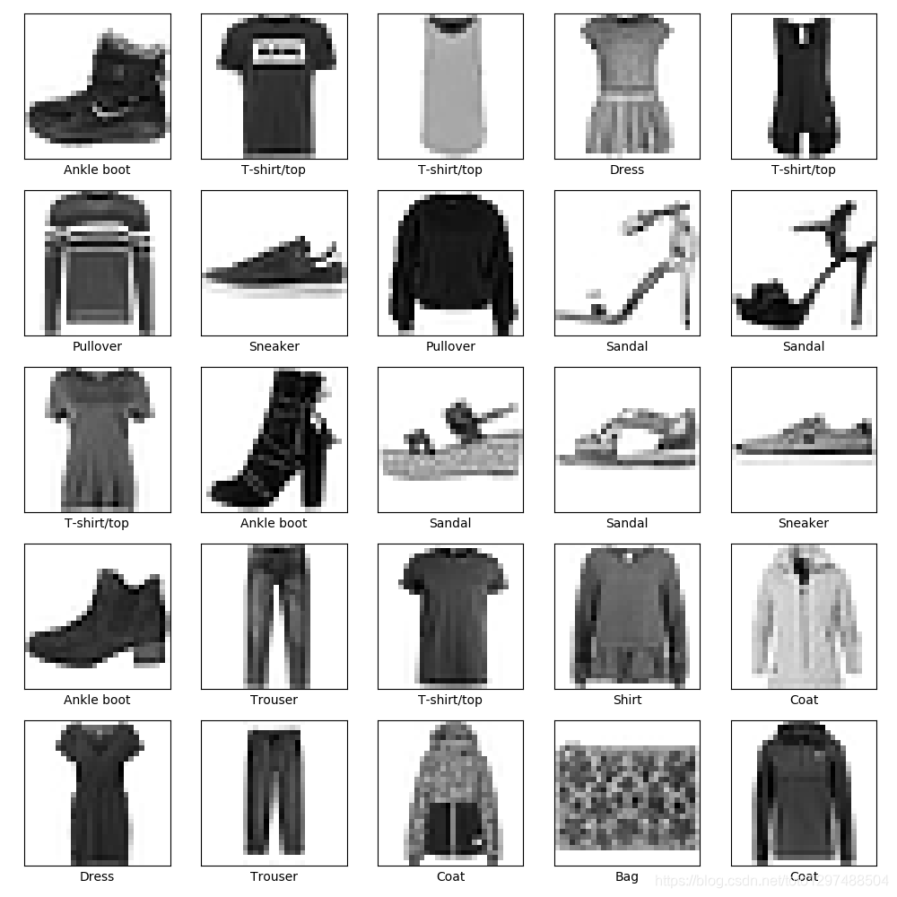
以验证数据的格式是否正确，并且您已经准备好构建和训练网络，让我们从训练集中展示开始的25张图片和在它下面展示每个分类的名称。

plt.figure(figsize=(10,10))
for i in range(25):
    plt.subplot(5,5,i+1)
    plt.xticks([])
    plt.yticks([])
    plt.grid(False)
    plt.imshow(train_images[i], cmap=plt.cm.binary)
    plt.xlabel(class_names[train_labels[i]])
plt.show()

显示结果：

1.3.1.4.构建模型

构建神经网络需要配置模型的层，然后编译模型。

1.3.1.4.1.设置层

神经网络的基本组成部分是层。层从输入给它们的数据中提取特征。这些特征对于手头上的问题是很有意义的。
大多数深度学习都是由一些层连接在一起的。大多数层，例如tf.keras.layers.Dense，拥有在学习训练中的参数。

model = keras.Sequential([
    keras.layers.Flatten(input_shape=(28,28)),
    keras.layers.Dense(128,activation='relu'),
    keras.layers.Dense(10)
])

在这个网络中第一层中， tf.keras.layers.Flatten，将图像格式从二维数组(28×28像素)转换为一维数组(28 * 28 = 784像素)。可以将这一层看作是将图像中的像素行展开并排列起来。这一层没有深度学习所需的参数。它只是重新格式化数据。

在像素值被flattened之后，这个网络由两个tf.keras.layers.Dense层的序列组成。它们是紧密相连或完全相连的神经层。这个第一个Dense层有128个节点（或者说神经元），第二个(也是最后一个)层返回长度为10的logits数组。每个节点包含一个分数，这个值表示当前图片属于这个10个分类中的一个的分值。

1.3.1.4.2.编译模型

在模型准备好训练之前，它需要一些更多的设置。在模型训练过程中这些参数被添加进去：
损失函数（Loss function）—这可以衡量模型在训练期间的准确性，您想最小化这个函数，以便将模型“引导”到正确的方向
优化器（Optimizer）— 这就是模型如何根据它看到的数据和它的损失函数进行更新.
Metrics—用于监控训练和测试步骤。下面的例子使用accuracy,即图片被正确分类的分数。

model.compile(optimizer='adam',
              loss=tf.keras.losses.SparseCategoricalCrossentropy(from_logits=True),
              metrics=['accuracy'])

1.3.1.5.训练模型

训练神经网络模型需要以下步骤：
1、将训练数据输入模型。在这个例子中，训练数据在train_images和train_labels数组中。
2、模型学习去关联图像和标签labels（目标值）
3、您要求模型对测试集进行预测。—在这个例子中，这里测试集即test_images数组。
4、验证预测是否与test_labels数组中的标签匹配。

1.3.1.5.1.Fit模型

调用model.fit方法开始训练模型。之所以这么说，是因为它使模型与训练数据“吻合”。

model.fit(train_images,train_labels,epochs=10)

输出结果：

Epoch 1/10
1875/1875 [==============================] - 3s 2ms/step - loss: 0.4957 - accuracy: 0.8262
Epoch 2/10
1875/1875 [==============================] - 3s 2ms/step - loss: 0.3758 - accuracy: 0.8652
Epoch 3/10
1875/1875 [==============================] - 3s 2ms/step - loss: 0.3373 - accuracy: 0.8766
Epoch 4/10
1875/1875 [==============================] - 3s 2ms/step - loss: 0.3112 - accuracy: 0.8859
Epoch 5/10
1875/1875 [==============================] - 3s 1ms/step - loss: 0.2968 - accuracy: 0.8896
Epoch 6/10
1875/1875 [==============================] - 3s 2ms/step - loss: 0.2820 - accuracy: 0.8956
Epoch 7/10
1875/1875 [==============================] - 3s 1ms/step - loss: 0.2700 - accuracy: 0.9002
Epoch 8/10
1875/1875 [==============================] - 3s 2ms/step - loss: 0.2577 - accuracy: 0.9030
Epoch 9/10
1875/1875 [==============================] - 3s 2ms/step - loss: 0.2497 - accuracy: 0.9060
Epoch 10/10
1875/1875 [==============================] - 3s 2ms/step - loss: 0.2385 - accuracy: 0.9106

作为模型训练，损失值和精确值被显示出来了。该模型对训练数据的准确率约为0.91 (91%)。

1.3.1.5.2.评估精确度

接下来，比较模型在测试数据集上的表现:

test_loss,test_acc = model.evaluate(test_images,test_labels,verbose=2)
print('\nTest accuracy:',test_acc)

输出结果：

313/313 - 0s - loss: 0.3528 - accuracy: 0.8791
Test accuracy: 0.8791000247001648

结果是测试数据集上的准确性比训练数据集上的准确性稍低，训练准确度和测试准确度之间的差距代表过拟合。当机器学习模型在新的、以前没有看到的输入上的表现不如在训练数据上的表现时，就会发生过拟合。过度拟合的模型“记忆”了训练数据集中的噪音和细节，从而对模型在新数据上的性能产生负面影响。欲了解更多信息，请参阅以下内容:
Demonstrate overfitting

Strategies to prevent overfitting

1.3.1.6.得出预测结果

通过训练模型，您可以使用它来对一些图像进行预测。模型的线性输出，logits。附加一个softmax层转换logits为概率，这个是一个更容易理解的数据。

probability_model = tf.keras.Sequential([model, tf.keras.layers.Softmax()])
predictions = probability_model.predict(test_images)

这里，模型已经对测试集中的每一张图像的标签进行了预测，让我们看一下第一个预测:

print(predictions[0])

输出结果为：

[1.9066751e-10 2.8168485e-12 2.6482936e-13 1.2655502e-12 3.0858400e-09
 1.4370863e-04 8.8831733e-09 6.9896835e-03 6.6860224e-09 9.9286664e-01]

预测是一个包含10个数字的数组，它们代表了模型的“confidence”，即图像对应着10种不同的服装（即是10种分类中每个分类的概率）。你可以看到哪个标签的置信度最高。

np.argmax(predictions[0])   #即最大可能的分类（目标值）

输出结果为：

9

所以，模特最自信的认为这是一双脚踝靴（Ankle boot）

绘制图表，看看10个类预测的全部集合。

def plot_image(i, predictions_array, true_label, img):
  predictions_array, true_label, img = predictions_array, true_label[i], img[i]
  plt.grid(False)
  plt.xticks([])
  plt.yticks([])

  plt.imshow(img, cmap=plt.cm.binary)

  predicted_label = np.argmax(predictions_array)
  if predicted_label == true_label:
    color = 'blue'
  else:
    color = 'red'

  plt.xlabel("{} {:2.0f}% ({})".format(class_names[predicted_label],
                                100*np.max(predictions_array),
                                class_names[true_label]),
                                color=color)

def plot_value_array(i, predictions_array, true_label):
  predictions_array, true_label = predictions_array, true_label[i]
  plt.grid(False)
  plt.xticks(range(10))
  plt.yticks([])
  thisplot = plt.bar(range(10), predictions_array, color="#777777")
  plt.ylim([0, 1])
  predicted_label = np.argmax(predictions_array)

  thisplot[predicted_label].set_color('red')
  thisplot[true_label].set_color('blue')

1.3.1.6.1.验证预测结果

通过训练模型，您可以使用它来对一些图像进行预测。

让我们看看第0个图像、预测和预测数组， 正确的预测标签为蓝色，错误的预测标签为红色。该数字给出了预测标签的百分比(满分100)

i = 0
plt.figure(figsize=(6,3))
plt.subplot(1,2,1)
plot_image(i, predictions[i], test_labels, test_images)
plt.subplot(1,2,2)
plot_value_array(i, predictions[i],  test_labels)
plt.show()

再如，预测错了的案例：

i = 12
plt.figure(figsize=(6,3))
plt.subplot(1,2,1)
plot_image(i, predictions[i], test_labels, test_images)
plt.subplot(1,2,2)
plot_value_array(i, predictions[i],  test_labels)
plt.show()

让我们用他们的预测画几个图像。注意，即使非常自信，模型也可能出错。

# Plot the first X test images, their predicted labels, and the true labels.
# Color correct predictions in blue and incorrect predictions in red.
num_rows = 5
num_cols = 3
num_images = num_rows*num_cols
plt.figure(figsize=(2*2*num_cols, 2*num_rows))
for i in range(num_images):
  plt.subplot(num_rows, 2*num_cols, 2*i+1)
  plot_image(i, predictions[i], test_labels, test_images)
  plt.subplot(num_rows, 2*num_cols, 2*i+2)
  plot_value_array(i, predictions[i], test_labels)
plt.tight_layout()
plt.show()

1.3.1.7.使用训练过的模型

最后，利用训练好的模型对单幅图像进行预测。

# Grab an image from the test dataset.
img = test_images[1]

print(img.shape)

输出结果为：

(28, 28)

tf.keras模型经过优化，可以立即对一批或一批示例进行预测,因此，即使你使用一个单一的图像，你需要添加到一个列表:

# Add the image to a batch where it's the only member
img = (np.expand_dims(img,0))
print(img.shape)

输出结果：

(1, 28, 28)

接着预测这个图片的正确结果：

predictions_single = probability_model.predict(img)
print(predictions_single)

输出结果：

[[1.1291439e-04 1.2360411e-12 9.9952698e-01 1.9153010e-09 2.9750227e-04
  2.1691890e-14 6.2605846e-05 1.1370566e-18 8.4102066e-11 1.2200014e-16]]

plot_value_array(1, predictions_single[0], test_labels)
_ = plt.xticks(range(10), class_names, rotation=45)

keras.Model.predict 返回列表的列表，这个列表是每个图像在批数据中的一个列表。抓取批处理中我们的(唯一的)图像的预测：

np.argmax(predictions_single[0])

输出结果是：

2

所有代码如下：

# -*- coding: UTF-8 -*-

# TensorFlow and tf.keras
import tensorflow as tf
from tensorflow import keras

# Helper libraries
import numpy as np
import matplotlib.pyplot as plt

print(tf.__version__)

fashion_mnist = keras.datasets.fashion_mnist
(train_images, train_labels), (test_images, test_labels) = fashion_mnist.load_data()

class_names = ['T-shirt/top', 'Trouser', 'Pullover', 'Dress', 'Coat',
               'Sandal', 'Shirt', 'Sneaker', 'Bag', 'Ankle boot']

print(train_images.shape)
print(train_labels)
print(len(train_labels))

print(test_images.shape)
print(len(test_labels))

print(train_images[0])

plt.figure()
plt.imshow(train_images[0])
plt.colorbar()
plt.grid(False)
plt.show()

train_images = train_images / 255.0
test_images = test_images / 255.0

plt.figure(figsize=(10,10))
for i in range(25):
    plt.subplot(5,5,i+1)
    plt.xticks([])
    plt.yticks([])
    plt.grid(False)
    plt.imshow(train_images[i], cmap=plt.cm.binary)
    plt.xlabel(class_names[train_labels[i]])
plt.show()

model = keras.Sequential([
    keras.layers.Flatten(input_shape=(28,28)),
    keras.layers.Dense(128,activation='relu'),
    keras.layers.Dense(10)
])

model.compile(optimizer='adam',
              loss=tf.keras.losses.SparseCategoricalCrossentropy(from_logits=True),
              metrics=['accuracy'])

model.fit(train_images,train_labels,epochs=10)

test_loss,test_acc = model.evaluate(test_images,test_labels,verbose=2)
print('\nTest accuracy:',test_acc)

probability_model = tf.keras.Sequential([model, tf.keras.layers.Softmax()])
predictions = probability_model.predict(test_images)
print(predictions[0])

print(np.argmax(predictions[0]))

def plot_image(i, predictions_array, true_label, img):
  predictions_array, true_label, img = predictions_array, true_label[i], img[i]
  plt.grid(False)
  plt.xticks([])
  plt.yticks([])

  plt.imshow(img, cmap=plt.cm.binary)

  predicted_label = np.argmax(predictions_array)
  if predicted_label == true_label:
    color = 'blue'
  else:
    color = 'red'

  plt.xlabel("{} {:2.0f}% ({})".format(class_names[predicted_label],
                                100*np.max(predictions_array),
                                class_names[true_label]),
                                color=color)

def plot_value_array(i, predictions_array, true_label):
  predictions_array, true_label = predictions_array, true_label[i]
  plt.grid(False)
  plt.xticks(range(10))
  plt.yticks([])
  thisplot = plt.bar(range(10), predictions_array, color="#777777")
  plt.ylim([0, 1])
  predicted_label = np.argmax(predictions_array)

  thisplot[predicted_label].set_color('red')
  thisplot[true_label].set_color('blue')

i = 0
plt.figure(figsize=(6,3))
plt.subplot(1,2,1)
plot_image(i, predictions[i], test_labels, test_images)
plt.subplot(1,2,2)
plot_value_array(i, predictions[i],  test_labels)
plt.show()

i = 12
plt.figure(figsize=(6,3))
plt.subplot(1,2,1)
plot_image(i, predictions[i], test_labels, test_images)
plt.subplot(1,2,2)
plot_value_array(i, predictions[i],  test_labels)
plt.show()



# Plot the first X test images, their predicted labels, and the true labels.
# Color correct predictions in blue and incorrect predictions in red.
num_rows = 5
num_cols = 3
num_images = num_rows*num_cols
plt.figure(figsize=(2*2*num_cols, 2*num_rows))
for i in range(num_images):
  plt.subplot(num_rows, 2*num_cols, 2*i+1)
  plot_image(i, predictions[i], test_labels, test_images)
  plt.subplot(num_rows, 2*num_cols, 2*i+2)
  plot_value_array(i, predictions[i], test_labels)
plt.tight_layout()
plt.show()


# Grab an image from the test dataset.
img = test_images[1]

print(img.shape)


# Add the image to a batch where it's the only member
img = (np.expand_dims(img,0))
print(img.shape)

predictions_single = probability_model.predict(img)
print(predictions_single)

plot_value_array(1, predictions_single[0], test_labels)
_ = plt.xticks(range(10), class_names, rotation=45)


print(np.argmax(predictions_single[0]))

官网还没出来中文版，自己翻译和整理，打个赏呗，您的支持是我坚持写好博文的动力