对于大多数的个人学习小伙伴来说,无法拥有一台性能超强的深度学习主机,更没有运算超群的服务器来供自己训练模型,但是又不得不对进行训练时,矛盾就产生了!
在深度学习训练中,我们经常遇到 GPU 的内存太小的问题,如果我们的数据量比较大,别说大批量(large batch size)训练了,有时候甚至连一个训练样本都放不下。但是随机梯度下降(SGD)中,如果能使用更大的 Batch Size 训练,一般能得到更好的结果。
那么问题来了:当 GPU 的内存不够时,如何使用大批量(large batch size)样本来训练神经网络呢?
这篇文章将以 PyTorch 为例,讲解一下几点:
- 当 GPU 的内存小于 Batch Size 的训练样本,或者甚至连一个样本都塞不下的时候,怎么用单个或多个 GPU 进行训练?
- 怎么尽量高效地利用多 GPU?
1、单个或多个 GPU 进行大批量训练
如果你也遇到过 CUDA RuntimeError: out of memory 的错误,那么说明你也遇到了这个问题。

PyTorch 的开发人员都出来了,估计一脸黑线:兄弟,这不是 bug,是你内存不够…
有一个方法可以解决这个问题:
梯度累加(accumulating gradients)。
一般在 PyTorch 中,我们是这样来更新梯度的:
predictions = model(inputs)               			# 前向计算
loss = loss_function(predictions, labels) 			# 计算损失函数
loss.backward()                           			# 后向计算梯度
optimizer.step()                          			# 优化器更新梯度
predictions = model(inputs)               			# 用更新过的参数值进行下一次前向计算
在上看的代码注释中,在计算梯度的 loss.backward() 操作中,每个参数的梯度被计算出来后,都被存储在各个参数对应的一个张量里:parameter.grad。然后优化器就会根据这个来更新每个参数的值,就是 optimizer.step()。
而梯度累加(accumulating gradients)的基本思想就是, 在优化器更新参数前,也就是执行 optimizer.step() 前,我们进行多次梯度计算,保存在 parameter.grad 中,然后累加梯度再更新。这个在 PyTorch 中特别容易实现,因为 PyTorch 中,梯度值本身会保留,除非我们调用 model.zero_grad() or optimizer.zero_grad()。
下面是一个梯度累加的例子,其中 accumulation_steps 就是要累加梯度的循环数:
model.zero_grad()                                   # 重置保存梯度值的张量
for i, (inputs, labels) in enumerate(training_set):
    predictions = model(inputs)                     # 前向计算
    loss = loss_function(predictions, labels)       # 计算损失函数
    loss = loss / accumulation_steps                # 对损失正则化 (如果需要平均所有损失)
    loss.backward()                                 # 计算梯度
    if (i 1) % accumulation_steps == 0:             # 重复多次前面的过程
        optimizer.step()                            # 更新梯度
        model.zero_grad()                           # 重置梯度
2、如果连一个样本都不放下怎么办?
如果样本特别大,别说 batch training,要是 GPU 的内存连一个样本都不下怎么办呢?
答案是使用梯度检查点(gradient-checkpoingting),用计算量来换内存。
基本思想就是,在反向传播的过程中,把梯度切分成几部分,分别对网络上的部分参数进行更新(见下图)。但这种方法的速度很慢,因为要增加额外的计算量。但在某些例子上又很有用,比如训练长序列的 RNN 模型等。
可以参考 PyTorch 官方文档对 Checkpoint 的描述:https://pytorch.org/docs/stable/checkpoint.html
TORCH.UTILS.CHECKPOINT
NOTE:
Checkpointing is implemented by rerunning a forward-pass segment for each checkpointed segment during backward. This can cause persistent states like the RNG state to be advanced than they would without checkpointing. By default, checkpointing includes logic to juggle the RNG state such that checkpointed passes making use of RNG (through dropout for example) have deterministic output as compared to non-checkpointed passes. The logic to stash and restore RNG states can incur a moderate performance hit depending on the runtime of checkpointed operations. If deterministic output compared to non-checkpointed passes is not required, supply preserve_rng_state=False to checkpoint or checkpoint_sequential to omit stashing and restoring the RNG state during each checkpoint.
The stashing logic saves and restores the RNG state for the current device and the device of all cuda Tensor arguments to the run_fn. However, the logic has no way to anticipate if the user will move Tensors to a new device within the run_fn itself. Therefore, if you move Tensors to a new device (“new” meaning not belonging to the set of [current device + devices of Tensor arguments]) within run_fn, deterministic output compared to non-checkpointed passes is never guaranteed.
-
torch.utils.checkpoint.checkpoint(function, *args, **kwargs)
Checkpoint a model or part of the model
Checkpointing works by trading compute for memory. Rather than storing all intermediate activations of the entire computation graph for computing backward, the checkpointed part does not save intermediate activations, and instead recomputes them in backward pass. It can be applied on any part of a model.
Specifically, in the forward pass, function will run in torch.no_grad() manner, i.e., not storing the intermediate activations. Instead, the forward pass saves the inputs tuple and the function parameter. In the backwards pass, the saved inputs and function is retrieved, and the forward pass is computed on function again, now tracking the intermediate activations, and then the gradients are calculated using these activation values.
WARNING:
Checkpointing doesn’t work with torch.autograd.grad(), but only with torch.autograd.backward().WARNING:
If function invocation during backward does anything different than the one during forward, e.g., due to some global variable, the checkpointed version won’t be equivalent, and unfortunately it can’t be detected.Parameters:
- function – describes what to run in the forward pass of the model or part of the model. It should also know how to handle the inputs passed as the tuple. For example, in LSTM, if user passes (activation, hidden), function should correctly use the first input as activation and the second input as hidden
- preserve_rng_state (bool, optional, default=True) – Omit stashing and restoring the RNG state during each checkpoint.
- args – tuple containing inputs to the function
Returns: Output of running function on *args
-
torch.utils.checkpoint.checkpoint_sequential(functions, segments, input, **kwargs)
A helper function for checkpointing sequential models.
Sequential models execute a list of modules/functions in order (sequentially). Therefore, we can divide such a model in various segments and checkpoint each segment. All segments except the last will run in torch.no_grad() manner, i.e., not storing the intermediate activations. The inputs of each checkpointed segment will be saved for re-running the segment in the backward pass.
See checkpoint() on how checkpointing works.WARNING:
Checkpointing doesn’t work with torch.autograd.grad(), but only with torch.autograd.backward().Parameters:
- functions – A torch.nn.Sequential or the list of modules or functions (comprising the model) to run sequentially.
- egments – Number of chunks to create in the model
- input – A Tensor that is input to functions
- preserve_rng_state (bool, optional, default=True) – Omit stashing and restoring the RNG state during each checkpoint.
Returns: Output of running functions sequentially on *inputs
Example:
>>> model = nn.Sequential(...)
>>> input_var = checkpoint_sequential(model, chunks, input_var)
3、多 GPU 训练方法
最简单、最暴力、最土豪的解决办法就是上多GPU进行训练。PyTorch 中多 GPU 训练的方法是使用 torch.nn.DataParallel。
非常简单,只需要一行代码:
torch.nn.DataParallel(module, device_ids=None, output_device=None, dim=0)
该函数实现了在module级别上的数据并行使用,注意batch size要大于GPU的数量。
参数 :
- module:需要多GPU训练的网络模型
- device_ids: GPU的编号(默认全部GPU)
- output_device:(默认是device_ids[0])
- dim:tensors被分散的维度,默认是0
device = torch.device("cuda:0" if torch.cuda.is_available() else "cpu")
定义device,其中需要注意的是“cuda:0” 代表起始的 device_id 为 0,如果直接是 “cuda”,同样默认是从 0 开始。可以根据实际需要修改起始位置,如 “cuda:1”。
model = Model()
if torch.cuda.device_count() > 1:
  model = nn.DataParallel(model,device_ids=[0,1,2])

model.to(device)
这里注意,如果是单GPU,直接model.to(device)就可以在单个GPU上训练,但如果是多个GPU就需要用到nn.DataParallel函数,然后在进行一次to(device)。
需要注意:device_ids的起始编号要与之前定义的device中的“cuda:0”相一致,不然会报错。
如果不定义device_ids,如model = nn.DataParallel(model),默认使用全部GPU。定义了device_ids就可以使用指定的GPU,但一定要注意与一开始定义device对应。
通过以上代码,就可以实现网络的多GPU训练。
parallel_model = torch.nn.DataParallel(model) # 就是这里!

predictions = parallel_model(inputs)          # 前向计算
loss = loss_function(predictions, labels)     # 计算损失函数
loss.mean().backward()                        # 计算多个GPU的损失函数平均值,计算梯度
optimizer.step()                              # 反向传播
predictions = parallel_model(inputs)
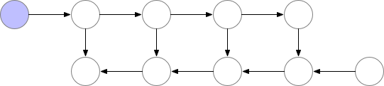
在使用torch.nn.DataParallel 的过程中,我们经常遇到一个问题:第一个GPU的计算量往往比较大。我们先来看一下多 GPU 的训练过程原理:

在上图第一行第四个步骤中,GPU-1 其实汇集了所有 GPU 的运算结果。这个对于多分类问题还好,但如果是自然语言处理模型就会出现问题,导致 GPU-1 汇集的梯度过大,直接爆掉。
那么就要想办法实现多 GPU 的负载均衡,方法就是让 GPU-1 不汇集梯度,而是保存在各个 GPU 上。这个方法的关键就是要分布化我们的损失函数,让梯度在各个 GPU 上单独计算和反向传播。这里又一个开源的实现:https://github.com/zhanghang1989/PyTorch-Encoding。这里是一个修改版,可以直接在我们的代码里调用。
实例:
from parallel import DataParallelModel, DataParallelCriterion

parallel_model = DataParallelModel(model)               # 并行化model
parallel_loss  = DataParallelCriterion(loss_function)   # 并行化损失函数

predictions = parallel_model(inputs)      				# 并行前向计算
                                          				# "predictions"是多个gpu的结果的元组
loss = parallel_loss(predictions, labels) 				# 并行计算损失函数
loss.backward()                           				# 计算梯度
optimizer.step()                          				# 反向传播
predictions = parallel_model(inputs)
如果你的网络输出是多个,可以这样分解:
output_1, output_2 = zip(*predictions)
如果有时候不想进行分布式损失函数计算,可以这样手动汇集所有结果:
gathered_predictions = parallel.gather(predictions)
下图展示了负载均衡以后的原理:
