梯度下降（一）：批梯度下降、随机梯度下降、小批量梯度下降、动量梯度下降、Nesterov加速梯度下降法 Matlab 可视化实现

前言

本文通过使用单变量线性回归模型讲解一些常见的梯度下降算法。为了更好的作对比，我们对参数设置了不同的学习率。

梯度下降法（GD / Gradient Descent）

梯度下降法(Gradient Descent)是一种常见的、用于寻找函数极小值的一阶迭代优化算法，又称为最速下降(Steepest Descent)，它是求解无约束最优化问题的一种常用方法。以下是梯度下降的基本公式：

$\theta := \theta - \frac{\partial J(\theta)}{\partial \theta}$
其中 $J(\theta)$ 是关于参数 $\theta$ 的损失函数， $\eta$ 是学习率(正标量)，也称为梯度下降的步长。由上述公式可知，梯度下降的想法是使得参数 $\theta$ 向着负梯度方向做更新迭代。

下面通过一个简单的例子来直观了解梯度下降的过程。假设 $J(\theta)$ 为关于 $\theta$ 的一元二次函数，即 $J(\theta) = \theta^2$。假设初始值为 $(\theta, J(\theta)) = (9,81)$， $\eta = 0.2。$对于第一次迭代，求取梯度为： $\frac{\partial J(\theta)}{\partial \theta} = 2\theta = 18$，更新 $\theta := \theta - \frac{\partial J(\theta)}{\partial \theta} = 9 - 0.2*18 = 5.4$。继续重复迭代步骤，最后函数将会趋于极值点 $x = 0$。

如下图所示，我们可以发现，随着梯度的不断减小，函数收敛越来越慢：

下面是该程序的matlab代码：

% writen by: Weichen Gu,   date: 4/18th/2020 
clc; clf; clear;
xdata = linspace(-10,10,1000);                   % x range
f = @(xdata)(xdata.^2);                         % Quadratic function - loss function

ydata = f(xdata);
plot(xdata,ydata,'c','linewidth',2);
title('y = x^2 (learning rate = 0.2)');
hold on;

x = [9 f(9)];            % Initial point
slope = inf;               % Slope
LRate = 0.2;               % Learning rate
slopeThresh = 0.0001;      % Slope threshold for iteration

plot(x(1),x(2),'r*');

while abs(slope) > slopeThresh
    [tmp,slope] = gradientDescent(x(1),f,LRate);
    x1 = [tmp f(tmp)];
    line([x(1),x1(1)],[x(2),x1(2)],'color','k','linestyle','--','linewidth',1);
    plot(x1(1),x1(2),'r*');
    legend('y = x^2');
    drawnow;
    x = x1;
end
hold off

function [xOut,slope] = gradientDescent(xIn,f, eta)
    syms x;
    slope = double(subs(diff(f(x)),xIn));
    xOut = xIn- eta*(slope);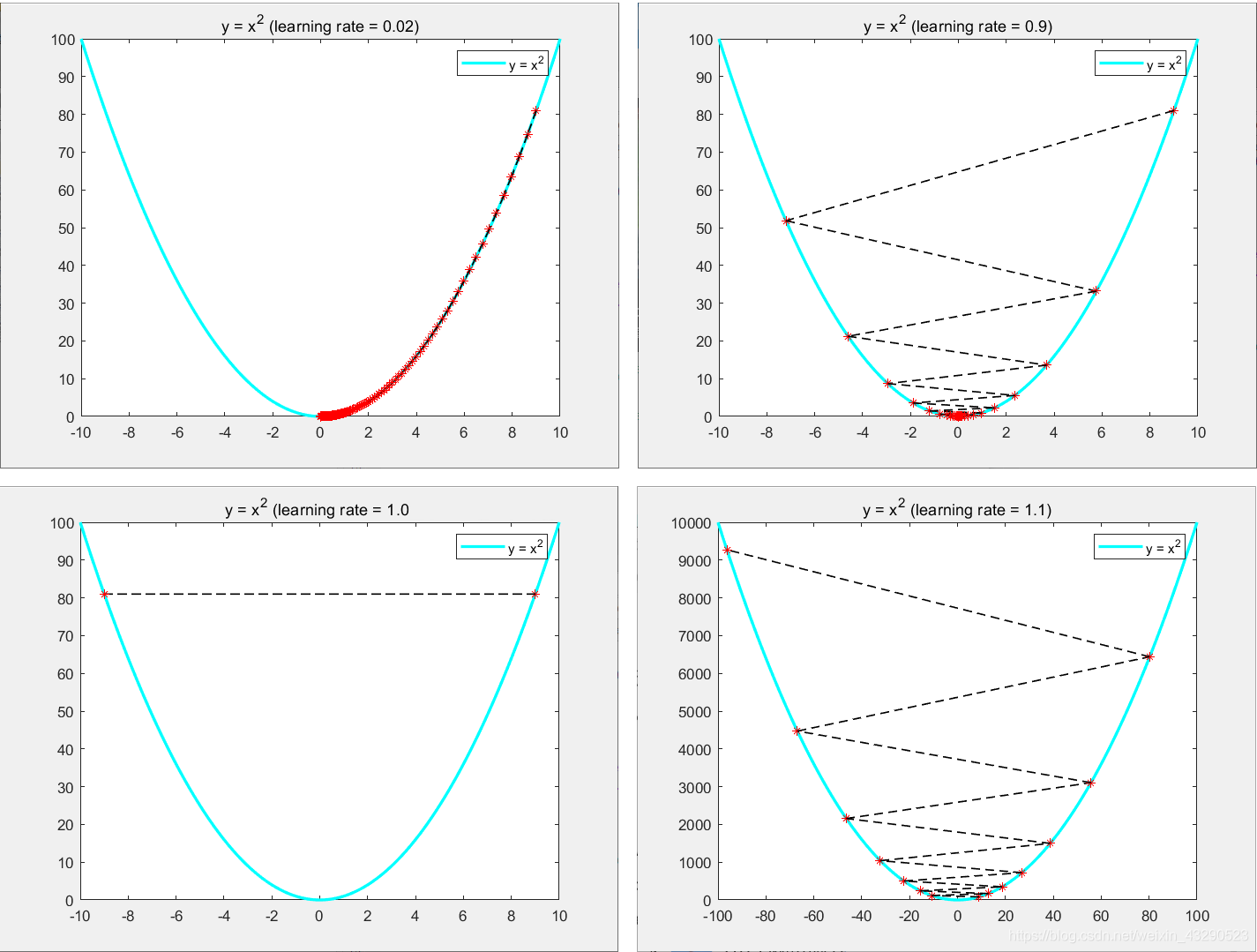
end

学习率决定了梯度下降的收敛速度，合适的学习率会使收敛速度得到一定的提高。我们应该避免过小或者过大的学习率：

• 学习率过小会导致函数收敛速度非常慢，所需迭代次数多，难以收敛。
• 学习率过大会导致梯度下降过程中出现震荡、不收敛甚至发散的情况。

如下图所示：

对于学习率，一开始可以设置较大的步长，然后再慢慢减小步长来调整收敛速度，但是实际过程中，设置最优的学习率一般来说是比较困难的。

同时我们应该知道，梯度下降是一种寻找函数极小值的方法，如下图，不同的初始点可能会获得不同的极小值：

单变量线性回归模型（Univariate Linear Regression）

下面我们通过使用吴恩达老师课程中的单变量线性回归(Univariate Linear Regression)模型来讲解几种梯度下降策略。如下公式：
$h_{\theta}(x) = \theta_0 x+\theta_1$

它是一种简单的线性拟合模型，并且目标函数为凸函数(根据一阶导二阶导性质)，所以对于梯度下降求得的极小值就是损失函数的最优解。下列公式为单变量线性回归模型的损失函数/目标函数：
$J(\theta_0,\theta_1) = \frac{1}{2m}\sum_{i = 1}^m(h_{\theta}(x^i)-y^i)^2$
其中 $h_\theta(x^{(i)})$是通过回归模型预测的输出。 $m$为样本个数。
我们的目标是求出使得目标函数最小的参数值
$(\hat\theta_0,\hat\theta_1) = \argmin_{\theta_0,\theta_1}J(\theta_0,\theta_1)$

对损失函数进行梯度求解，可得到：

$\frac{\partial J(\theta_0,\theta_1)}{\partial \theta_0} = \frac{1}{m}\sum_{i = 1}^m(\theta_0+\theta_1x^i -y^i)$ $\frac{\partial J(\theta_0,\theta_1)}{\partial \theta_1} = \frac{1}{m}\sum_{i = 1}^m(\theta_0+\theta_1x^i -y^i)x^i$

批梯度下降法（Batch GD / Batch Gradient Descent）

批梯度下降法根据整个数据集求取损失函数的梯度，来更新参数 $\theta$的值。公式如下：
$\theta := \theta - \eta\cdot\frac{1}{m}\sum_{i=1}^m\frac{\partial J(\theta,x^i,y^i)}{\partial \theta}$
优点：考虑到了全局数据，更新稳定，震荡小，每次更新都会朝着正确的方向。
缺点：如果数据集比较大，会造成大量时间和空间开销。

下图显示了通过批梯度下降进行拟合的结果。根据图像可看到，我们的线性回归模型逐渐拟合到了一个不错的结果。

下面给出matlab的代码：

% Writen by weichen GU, data 4/19th/2020
clear, clf, clc; 

data = linspace(-20,20,100);                    % x range
col = length(data);                             % Obtain the number of x
data = [data;0.5*data + wgn(1,100,1).*2+10];    % Generate dataset - y = 0.5 * x + wgn^2 + 10;
X = [ones(1, col); data(1,:)]';                 % X ->[1;X];

plot(data(1,:),data(2,:),'r.','MarkerSize',10); % Plot data
title('Data fiting using Univariate Linear Regression');
axis([-30,30,-10,30])
hold on;

theta =[0;0];           % Initialize parameters
LRate = [0.1; 0.002]; % Learning rate
thresh = 0.5;           % Threshold of loss for jumping iteration
iteration = 40;        % The number of teration

lineX = linspace(-30,30,100);
[row, col] = size(data)                     % Obtain the size of dataset
lineMy = [lineX;theta(1)*lineX+theta(2)];   % Fitting line
hLine = plot(lineMy(1,:),lineMy(2,:),'c','linewidth',2);  % draw fitting line

for iter = 1 : iteration
    delete(hLine)       % set(hLine,'visible','off')
    
    [thetaOut] = GD(X,data(2,:)',theta,LRate); % Gradient Descent algorithm
    theta = thetaOut;   % Update parameters(theta)
    
    loss = getLoss(X,data(2,:)',col,theta); % Obtain the loss 
    lineMy(2,:) = theta(2)*lineX+theta(1); % Fitting line
    hLine = plot(lineMy(1,:),lineMy(2,:),'c','linewidth',2); % draw fitting line
    
    drawnow()
    
    if(loss < thresh)
        break;
    end
end

hold off


function [thetaOut] = GD(X,Y,theta,LRate)
    dataSize = length(X);               % Obtain the number of data 
    dx = 1/dataSize*(X'*(X*theta-Y));   % Obtain the gradient
    thetaOut = theta -LRate.*dx;         % gradient descent method
end


function [Z] = getLoss(X,Y, num,theta)
    Z= 1/(2*num)*sum((X*theta-Y).^2);
end

我们希望可以直观的看到批梯度下降的过程，以便和后续的一些梯度下降算法作比较，于是我们将其三维可视化出来，画出其拟合图(1)、三维损失图(2)、等高线图(3)以及迭代损失图(4)：

根据上图可以看到，批梯度下降收敛稳定，震荡小。

这里给出具体matlab实现代码：

% Writen by weichen GU, data 4/19th/2020
clear, clf, clc;
data = linspace(-20,20,100);                    % x range
col = length(data);                             % Obtain the number of x
data = [data;0.5*data + wgn(1,100,1)+10];       % Generate dataset - y = 0.5 * x + wgn^2 + 10;
X = [ones(1, col); data(1,:)]';                 % X ->[1;X];

t1=-40:0.1:50;
t2=-4:0.1:4;
[meshX,meshY]=meshgrid(t1,t2);
meshZ = getTotalCost(X, data(2,:)', col, meshX,meshY);

theta =[-30;-4];        % Initialize parameters
LRate = [0.1; 0.002];   % Learning rate
thresh = 0.5;           % Threshold of loss for jumping iteration
iteration = 50;         % The number of teration

lineX = linspace(-30,30,100);
[row, col] = size(data)                                     % Obtain the size of dataset
lineMy = [lineX;theta(1)*lineX+theta(2)];                   % Fitting line
hLine = plot(lineMy(1,:),lineMy(2,:),'c','linewidth',2);    % draw fitting line

loss = getLoss(X,data(2,:)',col,theta);                     % Obtain current loss value

subplot(2,2,1);
plot(data(1,:),data(2,:),'r.','MarkerSize',10);
title('Data fiting using Univariate LR');
axis([-30,30,-10,30])
xlabel('x');
ylabel('y');
hold on;

% Draw 3d loss surfaces
subplot(2,2,2)
mesh(meshX,meshY,meshZ)
xlabel('θ_0');
ylabel('θ_1');
title('3D surfaces for loss')
hold on;
scatter3(theta(1),theta(2),loss,'r*');

% Draw loss contour figure
subplot(2,2,3)
contour(meshX,meshY,meshZ)
xlabel('θ_0');
ylabel('θ_1');
title('Contour figure for loss')
hold on;
plot(theta(1),theta(2),'r*')

% Draw loss with iteration
subplot(2,2,4)
hold on;
title('Loss when using Batch GD');
xlabel('iter');
ylabel('loss');
plot(0,loss,'b*');

set(gca,'XLim',[0 iteration]);
%set(gca,'YLim',[0 4000]);
hold on;

for iter = 1 : iteration
    delete(hLine) % set(hLine,'visible','off')
    
    [thetaOut] = GD(X,data(2,:)',theta,LRate); % Gradient Descent algorithm
    subplot(2,2,3);
    line([theta(1),thetaOut(1)],[theta(2),thetaOut(2)],'color','k')

    theta = thetaOut;
    loss = getLoss(X,data(2,:)',col,theta); % Obtain losw
    
    
    lineMy(2,:) = theta(2)*lineX+theta(1); % Fitting line
    subplot(2,2,1);
    hLine = plot(lineMy(1,:),lineMy(2,:),'c','linewidth',2); % draw fitting line
    %legend('training data','linear regression');
    
    subplot(2,2,2);
    scatter3(theta(1),theta(2),loss,'r*');
    
    subplot(2,2,3);
    plot(theta(1),theta(2),'r*')
    
    subplot(2,2,4)
    plot(iter,loss,'b*');
    
    drawnow();
    
    if(loss < thresh)
        break;
    end
end

hold off


function [Z] = getTotalCost(X,Y, num,meshX,meshY);
    [row,col] = size(meshX);
    Z = zeros(row, col);
    for i = 1 : row
        theta = [meshX(i,:); meshY(i,:)];
        Z(i,:) =  1/(2*num)*sum((X*theta-repmat(Y,1,col)).^2);   
    end

end

function [Z] = getLoss(X,Y, num,theta)
    Z= 1/(2*num)*sum((X*theta-Y).^2);
end

function [thetaOut] = GD(X,Y,theta,eta)
    dataSize = length(X);                       % Obtain the number of data
    dx = 1/dataSize.*(X'*(X*theta-Y));          % Obtain the gradient of Loss function
    thetaOut = theta -eta.*dx;                  % Update parameters(theta)
end

随机梯度下降法（SGD / Stochastic Gradient Descent）

因为批梯度下降所需要的时间空间成本大，我们考虑随机抽取一个样本来获取梯度，更新参数 $\theta$。其公式如下：
$\theta := \theta - \eta\cdot\frac{\partial J(\theta,x^i,y^i)}{\partial \theta}$步骤如下：

1. 随机打乱数据集。
2. 对于每个样本点，依次迭代更新参数 $\theta$。
3. 重复以上步骤直至损失足够小或到达迭代阈值。

优点：训练速度快，每次迭代只需要一个样本，相对于批梯度下降，总时间、空间开销小。
缺点：噪声大导致高方差。导致每次迭代并不一定朝着最优解收敛，震荡大。

下图直观显示了随机梯度下降的迭代过程：

下面给出随机梯度下降的matlab代码，因为它是小批量梯度下降的特殊情况(batchSize = 1)，所以我将小批量梯度下降的代码放在本章节，并设置batchSize = 1。

% Writen by weichen GU, data 4/19th/2020
clear, clf, clc;
data = linspace(-20,20,100);                    % x range
col = length(data);                             % Obtain the number of x
data = [data;0.5*data + wgn(1,100,1)+10];       % Generate dataset - y = 0.5 * x + wgn^2 + 10;
X = [ones(1, col); data(1,:)]';                 % X ->[1;X];

t1=-40:0.1:50;
t2=-4:0.1:4;
[meshX,meshY]=meshgrid(t1,t2);
meshZ = getTotalCost(X, data(2,:)', col, meshX,meshY);

theta =[-30;-4];        % Initialize parameters
LRate = [0.1; 0.002]  % Learning rate
thresh = 0.5;           % Threshold of loss for jumping iteration
iteration = 100;        % The number of teration

lineX = linspace(-30,30,100);
[row, col] = size(data)                                     % Obtain the size of dataset
lineMy = [lineX;theta(1)*lineX+theta(2)];                   % Fitting line
hLine = plot(lineMy(1,:),lineMy(2,:),'c','linewidth',2);    % draw fitting line

loss = getLoss(X,data(2,:)',col,theta);                     % Obtain current loss value

subplot(2,2,1);
plot(data(1,:),data(2,:),'r.','MarkerSize',10);
title('Data fiting using Univariate LR');
axis([-30,30,-10,30])
xlabel('x');
ylabel('y');
hold on;

% Draw 3d loss surfaces
subplot(2,2,2)
mesh(meshX,meshY,meshZ)
xlabel('θ_0');
ylabel('θ_1');
title('3D surfaces for loss')
hold on;
scatter3(theta(1),theta(2),loss,'r*');

% Draw loss contour figure
subplot(2,2,3)
contour(meshX,meshY,meshZ)
xlabel('θ_0');
ylabel('θ_1');
title('Contour figure for loss')
hold on;
plot(theta(1),theta(2),'r*')

% Draw loss with iteration
subplot(2,2,4)
hold on;
title('Loss when using SGD');
xlabel('iter');
ylabel('loss');
plot(0,loss,'b*');

set(gca,'XLim',[0 iteration]);
hold on;

batchSize = 1;
for iter = 1 : iteration
    delete(hLine) % set(hLine,'visible','off')

    
    %[thetaOut] = GD(X,data(2,:)',theta,LRate); % Gradient Descent algorithm
    [thetaOut] = MBGD(X,data(2,:)',theta,LRate,batchSize);
    subplot(2,2,3);
    line([theta(1),thetaOut(1)],[theta(2),thetaOut(2)],'color','k')

    theta = thetaOut;
    loss = getLoss(X,data(2,:)',col,theta); % Obtain losw
    
    
    lineMy(2,:) = theta(2)*lineX+theta(1); % Fitting line
    subplot(2,2,1);
    hLine = plot(lineMy(1,:),lineMy(2,:),'c','linewidth',2); % draw fitting line
    %legend('training data','linear regression');
    
    subplot(2,2,2);
    scatter3(theta(1),theta(2),loss,'r*');
    
    subplot(2,2,3);
    plot(theta(1),theta(2),'r*')
    
    
    subplot(2,2,4)
    plot(iter,loss,'b*');
    
    drawnow();
    
    if(loss < thresh)
        break;
    end
end

hold off


function [Z] = getTotalCost(X,Y, num,meshX,meshY);
    [row,col] = size(meshX);
    Z = zeros(row, col);
    for i = 1 : row
        theta = [meshX(i,:); meshY(i,:)];
        Z(i,:) =  1/(2*num)*sum((X*theta-repmat(Y,1,col)).^2);   
    end

end


function [Z] = getLoss(X,Y, num,theta)
    Z= 1/(2*num)*sum((X*theta-Y).^2);
end

function [thetaOut] = GD(X,Y,theta,eta)
    dataSize = length(X);                       % Obtain the number of data
    dx = 1/dataSize.*(X'*(X*theta-Y));          % Obtain the gradient of Loss function
    thetaOut = theta -eta.*dx;                  % Update parameters(theta)
end

% @ Depscription: 
%       Mini-batch Gradient Descent (MBGD)
%       Stochastic Gradient Descent(batchSize = 1) (SGD)
% @ param:
%       X - [1 X_] X_ is actual X; Y - actual Y
%       theta - theta for univariate linear regression y_pred = theta_0 + theta1*x
%       eta - learning rate;
%
function [thetaOut] = MBGD(X,Y,theta, eta,batchSize) 
    dataSize = length(X);           % obtain the number of data 
    k = fix(dataSize/batchSize);    % obtain the number of batch which has absolutely same size: k = batchNum-1;    
    batchIdx = randperm(dataSize);  % randomly sort for every epoch for achiving sample diversity
    
    batchIdx1 = reshape(batchIdx(1:k*batchSize),k,batchSize);   % batches which has absolutely same size
    batchIdx2 = batchIdx(k*batchSize+1:end);                    % ramained batch
    
    for i = 1 : k
        thetaOut = GD(X(batchIdx1(i,:),:),Y(batchIdx1(i,:)),theta,eta);
    end
    if(~isempty(batchIdx2))
        thetaOut = GD(X(batchIdx2,:),Y(batchIdx2),thetaOut,eta);
    end
end

小批量梯度下降（Mini Batch GD / Mini-batch Gradient Descent）

随机梯度下降收敛速度快，但是波动较大，在最优解处出现波动很难判断其是否收敛到一个合理的值。而批梯度下降稳定但是时空开销很大，针对于这种情况，我们引入小批量梯度下降对二者进行折衷，在每轮迭代过程中使用n个样本来训练参数：
$\theta := \theta - \eta\cdot\frac{1}{n}\sum_{i=1}^n\frac{\partial J(\theta,x^i,y^i)}{\partial \theta}$步骤如下：

1. 随机打乱数据集。
2. 将数据集分为 $\frac{m}{n}$个集合，如果有余，将剩余样本单独作为一个集合。
3. 依次对于这些集合做批梯度下降，更新参数 $\theta$。
4. 重复上述步骤，直至损失足够小或达到迭代阈值。

下图显示了小批量梯度下降的迭代过程，其中batchSize = 32。我们可以看到，小批量折衷了批梯度下降和随机梯度下降的特点，做到了相对来说收敛快、较稳定的结果。

这里附上小批量梯度下降的相关代码：

% Writen by weichen GU, data 4/19th/2020
clear, clf, clc;
data = linspace(-20,20,100);                    % x range
col = length(data);                             % Obtain the number of x
data = [data;0.5*data + wgn(1,100,1)+10];       % Generate dataset - y = 0.5 * x + wgn^2 + 10;
X = [ones(1, col); data(1,:)]';                 % X ->[1;X];

t1=-40:0.1:50;
t2=-4:0.1:4;
[meshX,meshY]=meshgrid(t1,t2);
meshZ = getTotalCost(X, data(2,:)', col, meshX,meshY);

theta =[-30;-4];        % Initialize parameters
LRate = [0.1; 0.002]  % Learning rate
thresh = 0.5;           % Threshold of loss for jumping iteration
iteration = 50;        % The number of teration

lineX = linspace(-30,30,100);
[row, col] = size(data)                                     % Obtain the size of dataset
lineMy = [lineX;theta(1)*lineX+theta(2)];                   % Fitting line
hLine = plot(lineMy(1,:),lineMy(2,:),'c','linewidth',2);    % draw fitting line

loss = getLoss(X,data(2,:)',col,theta);                     % Obtain current loss value

subplot(2,2,1);
plot(data(1,:),data(2,:),'r.','MarkerSize',10);
title('Data fiting using Univariate LR');
axis([-30,30,-10,30])
xlabel('x');
ylabel('y');
hold on;

% Draw 3d loss surfaces
subplot(2,2,2)
mesh(meshX,meshY,meshZ)
xlabel('θ_0');
ylabel('θ_1');
title('3D surfaces for loss')
hold on;
scatter3(theta(1),theta(2),loss,'r*');

% Draw loss contour figure
subplot(2,2,3)
contour(meshX,meshY,meshZ)
xlabel('θ_0');
ylabel('θ_1');
title('Contour figure for loss')
hold on;
plot(theta(1),theta(2),'r*')

% Draw loss with iteration
subplot(2,2,4)
hold on;
title('Loss when using Mini-Batch GD');
xlabel('iter');
ylabel('loss');
plot(0,loss,'b*');

set(gca,'XLim',[0 iteration]);
%set(gca,'YLim',[0 4000]);
hold on;

batchSize = 32;
for iter = 1 : iteration
    delete(hLine) % set(hLine,'visible','off')

    
    %[thetaOut] = GD(X,data(2,:)',theta,LRate); % Gradient Descent algorithm
    [thetaOut] = MBGD(X,data(2,:)',theta,LRate,batchSize);
    subplot(2,2,3);
    line([theta(1),thetaOut(1)],[theta(2),thetaOut(2)],'color','k')

    theta = thetaOut;
    loss = getLoss(X,data(2,:)',col,theta); % Obtain losw
    
    
    lineMy(2,:) = theta(2)*lineX+theta(1); % Fitting line
    subplot(2,2,1);
    hLine = plot(lineMy(1,:),lineMy(2,:),'c','linewidth',2); % draw fitting line
    %legend('training data','linear regression');
    
    subplot(2,2,2);
    scatter3(theta(1),theta(2),loss,'r*');
    
    subplot(2,2,3);
    plot(theta(1),theta(2),'r*')
    
    
    subplot(2,2,4)
    plot(iter,loss,'b*');
    
    drawnow();
    
    if(loss < thresh)
        break;
    end
end

hold off


function [Z] = getTotalCost(X,Y, num,meshX,meshY);
    [row,col] = size(meshX);
    Z = zeros(row, col);
    for i = 1 : row
        theta = [meshX(i,:); meshY(i,:)];
        Z(i,:) =  1/(2*num)*sum((X*theta-repmat(Y,1,col)).^2);   
    end

end


function [Z] = getLoss(X,Y, num,theta)
    Z= 1/(2*num)*sum((X*theta-Y).^2);
end

function [thetaOut] = GD(X,Y,theta,eta)
    dataSize = length(X);                       % Obtain the number of data
    dx = 1/dataSize.*(X'*(X*theta-Y));          % Obtain the gradient of Loss function
    thetaOut = theta -eta.*dx;                  % Update parameters(theta)
end

% @ Depscription: 
%       Mini-batch Gradient Descent (MBGD)
%       Stochastic Gradient Descent(batchSize = 1) (SGD)
% @ param:
%       X - [1 X_] X_ is actual X; Y - actual Y
%       theta - theta for univariate linear regression y_pred = theta_0 + theta1*x
%       eta - learning rate;
%
function [thetaOut] = MBGD(X,Y,theta, eta,batchSize) 
    dataSize = length(X);           % obtain the number of data 
    k = fix(dataSize/batchSize);    % obtain the number of batch which has absolutely same size: k = batchNum-1;    
    batchIdx = randperm(dataSize);  % randomly sort for every epoch for achiving sample diversity
    
    batchIdx1 = reshape(batchIdx(1:k*batchSize),k,batchSize);   % batches which has absolutely same size
    batchIdx2 = batchIdx(k*batchSize+1:end);                    % ramained batch
    
    for i = 1 : k
        thetaOut = GD(X(batchIdx1(i,:),:),Y(batchIdx1(i,:)),theta,eta);
    end
    if(~isempty(batchIdx2))
        thetaOut = GD(X(batchIdx2,:),Y(batchIdx2),thetaOut,eta);
    end
end

动量梯度下降（Momentum / Gradient Descent with Momentum）

动量梯度下降通过指数加权平均(Exponentially weighted moving averages)策略，使用之前梯度信息修正当前梯度，来加速参数学习。这里我们令梯度项
$\frac{1}{m}\sum_{i=1}^m\frac{\partial J(\theta,x^i,y^i)}{\partial \theta} = \nabla_\theta J(\theta)$则梯度下降可以简化表示为
$\theta := \theta - \eta\cdot\nabla_\theta J(\theta)$
对于动量梯度下降，初始化动量项 $m = 0$，更新迭代公式如下
$m := \gamma\cdot m + \eta\cdot\nabla_\theta J(\theta)$ $\theta :=\theta - m$
其中 $m$为动量梯度下降的动量项，且初始化为0； $\gamma$是关于动量项的超参数一般取小于等于0.9。我们可以发现，越是远离当前点的梯度信息，对于当前梯度的贡献越小。

优点：通过过去梯度信息来优化下降速度，如果当前梯度与之前梯度方向一致时候，收敛速度得到加强，反之则减弱。换句话说，加快收敛同时减小震荡，分别对应图中 $\theta_0$ 与 $\theta_1$ 方向。
缺点：可能在下坡过程中累计动量太大，冲过极小值点。

下图直观显示动量梯度下降迭代过程。

这里附上动量梯度下降的相关代码：

% Writen by weichen GU, data 4/19th/2020
clear, clf, clc;
data = linspace(-20,20,100);                    % x range
col = length(data);                             % Obtain the number of x
data = [data;0.5*data + wgn(1,100,1)+10];       % Generate dataset - y = 0.5 * x + wgn^2 + 10;
X = [ones(1, col); data(1,:)]';                 % X ->[1;X];

t1=-40:0.1:50;
t2=-4:0.1:4;
[meshX,meshY]=meshgrid(t1,t2);
meshZ = getTotalCost(X, data(2,:)', col, meshX,meshY);

theta =[-30;-4];        % Initialize parameters
LRate = [0.1; 0.002]  % Learning rate
thresh = 0.5;           % Threshold of loss for jumping iteration
iteration = 50;        % The number of teration

lineX = linspace(-30,30,100);
[row, col] = size(data)                                     % Obtain the size of dataset
lineMy = [lineX;theta(1)*lineX+theta(2)];                   % Fitting line
hLine = plot(lineMy(1,:),lineMy(2,:),'c','linewidth',2);    % draw fitting line

loss = getLoss(X,data(2,:)',col,theta);                     % Obtain current loss value

subplot(2,2,1);
plot(data(1,:),data(2,:),'r.','MarkerSize',10);
title('Data fiting using Univariate LR');
axis([-30,30,-10,30])
xlabel('x');
ylabel('y');
hold on;

% Draw 3d loss surfaces
subplot(2,2,2)
mesh(meshX,meshY,meshZ)
xlabel('θ_0');
ylabel('θ_1');
title('3D surfaces for loss')
hold on;
scatter3(theta(1),theta(2),loss,'r*');

% Draw loss contour figure
subplot(2,2,3)
contour(meshX,meshY,meshZ)
xlabel('θ_0');
ylabel('θ_1');
title('Contour figure for loss')
hold on;
plot(theta(1),theta(2),'r*')

% Draw loss with iteration
subplot(2,2,4)
hold on;
title('Loss when using Momentum GD');
xlabel('iter');
ylabel('loss');
plot(0,loss,'b*');

set(gca,'XLim',[0 iteration]);

hold on;

batchSize = 32;
grad = 0; gamma = 0.5;

for iter = 1 : iteration
    delete(hLine) % set(hLine,'visible','off')

    
    %[thetaOut] = GD(X,data(2,:)',theta,LRate); % Gradient Descent algorithm
    %[thetaOut] = MBGD(X,data(2,:)',theta,LRate,20);
    [thetaOut,grad] = MBGDM(X,data(2,:)',theta,LRate,batchSize,grad,gamma);
    subplot(2,2,3);
    line([theta(1),thetaOut(1)],[theta(2),thetaOut(2)],'color','k')

    theta = thetaOut;
    loss = getLoss(X,data(2,:)',col,theta); % Obtain losw
    
    
    lineMy(2,:) = theta(2)*lineX+theta(1); % Fitting line
    subplot(2,2,1);
    hLine = plot(lineMy(1,:),lineMy(2,:),'c','linewidth',2); % draw fitting line
    %legend('training data','linear regression');
    
    subplot(2,2,2);
    scatter3(theta(1),theta(2),loss,'r*');
    
    subplot(2,2,3);
    plot(theta(1),theta(2),'r*')
    
    
    subplot(2,2,4)
    plot(iter,loss,'b*');

    drawnow();
    
    if(loss < thresh)
        break;
    end
end

hold off


function [Z] = getTotalCost(X,Y, num,meshX,meshY);
    [row,col] = size(meshX);
    Z = zeros(row, col);
    for i = 1 : row
        theta = [meshX(i,:); meshY(i,:)];
        Z(i,:) =  1/(2*num)*sum((X*theta-repmat(Y,1,col)).^2);   
    end

end


function [Z] = getLoss(X,Y, num,theta)
    Z= 1/(2*num)*sum((X*theta-Y).^2);
end

function [thetaOut] = GD(X,Y,theta,eta)
    dataSize = length(X);                       % Obtain the number of data
    dx = 1/dataSize.*(X'*(X*theta-Y));          % Obtain the gradient of Loss function
    thetaOut = theta -eta.*dx;                  % Update parameters(theta)
end
% Gradient Descent with Momentum
function [thetaOut, momentum] = GDM(X,Y,theta,eta,momentum,gamma)
    dataSize = length(X);                       % Obtain the number of data
    dx = 1/dataSize.*(X'*(X*theta-Y));          % Obtain the gradient of Loss function
    momentum = gamma*momentum +eta.*dx;         % Obtain the momentum of gradient
    thetaOut = theta - momentum;                % Update parameters(theta)
end

% @ Depscription: 
%       Mini-batch Gradient Descent (MBGD)
%       Stochastic Gradient Descent(batchSize = 1) (SGD)
% @ param:
%       X - [1 X_] X_ is actual X; Y - actual Y
%       theta - theta for univariate linear regression y_pred = theta_0 + theta1*x
%       eta - learning rate;
%
function [thetaOut] = MBGD(X,Y,theta, eta,batchSize) 
    dataSize = length(X);           % obtain the number of data 
    k = fix(dataSize/batchSize);    % obtain the number of batch which has absolutely same size: k = batchNum-1;    
    batchIdx = randperm(dataSize);  % randomly sort for every epoch for achiving sample diversity
    
    batchIdx1 = reshape(batchIdx(1:k*batchSize),k,batchSize);   % batches which has absolutely same size
    batchIdx2 = batchIdx(k*batchSize+1:end);                    % ramained batch
    
    for i = 1 : k
        thetaOut = GD(X(batchIdx1(i,:),:),Y(batchIdx1(i,:)),theta,eta);
    end
    if(~isempty(batchIdx2))
        thetaOut = GD(X(batchIdx2,:),Y(batchIdx2),thetaOut,eta);
    end
end

function [thetaOut,grad] = MBGDM(X,Y,theta, eta,batchSize,grad,gamma) 
    dataSize = length(X);           % obtain the number of data 
    k = fix(dataSize/batchSize);    % obtain the number of batch which has absolutely same size: k = batchNum-1;    
    batchIdx = randperm(dataSize);  % randomly sort for every epoch for achiving sample diversity
    
    batchIdx1 = reshape(batchIdx(1:k*batchSize),k,batchSize);   % batches which has absolutely same size
    batchIdx2 = batchIdx(k*batchSize+1:end);                    % ramained batch
    
    for i = 1 : k
        [thetaOut,grad] = GDM(X(batchIdx1(i,:),:),Y(batchIdx1(i,:)),theta,eta,grad,gamma);
        
    end
    if(~isempty(batchIdx2))
        [thetaOut,grad] = GDM(X(batchIdx2,:),Y(batchIdx2),thetaOut,eta,grad,gamma);
    end
end

Nesterov加速梯度下降法（NAG / Nesterov Accelerated Gradient）

Nesterov加速梯度下降相比于动量梯度下降的区别是，通过使用未来梯度来更新动量。即将下一次的预测梯度 $\nabla_\theta J(\theta-\eta\cdot m)$考虑进来。其更新公式如下：
$m :=\gamma\cdot m+\eta\cdot\nabla_\theta J(\theta-\gamma\cdot m)$ $\theta := \theta - m$
对于公式理解如下图所示，

1. 对于起始点应用动量梯度下降，首先求得在该点处的带权梯度 $\eta\cdot\nabla_1$，通过与之前动量 $\gamma\cdot m$矢量加权，求得下一次的 $\theta$位置。
2. 对于起始点应用Nesterov加速梯度下降，首先通过先前动量求得 $\theta$的预测位置，再加上预测位置的带权梯度 $\gamma\cdot m$。

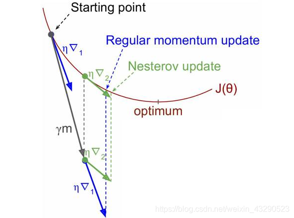
优点：

1. 相对于动量梯度下降法，因为NAG考虑到了未来预测梯度，收敛速度更快（如上图）。
2. 当更新幅度很大时，NAG可以抑制震荡。例如起始点在最优点的左侧←， $\gamma m$对应的值在最优点的右侧→，对于动量梯度而言，叠加 $\eta\nabla_1$使得迭代后的点更加远离最优点→→。而NAG首先跳到 $\gamma m$对应的值→，计算梯度为正，再叠加反方向的 $\eta\nabla_2$←，从而达到抑制震荡的目的。

下图直观显示了Nesterov加速梯度下降的迭代过程：

下面是Nesterov加速梯度下降的相关代码：

% Writen by weichen GU, data 4/19th/2020
clear, clf, clc;
data = linspace(-20,20,100);                    % x range
col = length(data);                             % Obtain the number of x
data = [data;0.5*data + wgn(1,100,1)+10];       % Generate dataset - y = 0.5 * x + wgn^2 + 10;
X = [ones(1, col); data(1,:)]';                 % X ->[1;X];

t1=-40:0.1:50;
t2=-4:0.1:4;
[meshX,meshY]=meshgrid(t1,t2);
meshZ = getTotalCost(X, data(2,:)', col, meshX,meshY);

theta =[-30;-4];        % Initialize parameters
LRate = [0.1; 0.002]  % Learning rate
thresh = 0.5;           % Threshold of loss for jumping iteration
iteration = 50;        % The number of teration

lineX = linspace(-30,30,100);
[row, col] = size(data)                                     % Obtain the size of dataset
lineMy = [lineX;theta(1)*lineX+theta(2)];                   % Fitting line
hLine = plot(lineMy(1,:),lineMy(2,:),'c','linewidth',2);    % draw fitting line

loss = getLoss(X,data(2,:)',col,theta);                     % Obtain current loss value

subplot(2,2,1);
plot(data(1,:),data(2,:),'r.','MarkerSize',10);
title('Data fiting using Univariate LR');
axis([-30,30,-10,30])
xlabel('x');
ylabel('y');
hold on;

% Draw 3d loss surfaces
subplot(2,2,2)
mesh(meshX,meshY,meshZ)
xlabel('θ_0');
ylabel('θ_1');
title('3D surfaces for loss')
hold on;
scatter3(theta(1),theta(2),loss,'r*');

% Draw loss contour figure
subplot(2,2,3)
contour(meshX,meshY,meshZ)
xlabel('θ_0');
ylabel('θ_1');
title('Contour figure for loss')
hold on;
plot(theta(1),theta(2),'r*')

% Draw loss with iteration
subplot(2,2,4)
hold on;
title('Loss when using NAG');
xlabel('iter');
ylabel('loss');
plot(0,loss,'b*');

set(gca,'XLim',[0 iteration]);

hold on;

batchSize = 32;
grad = 0; gamma = 0.5;

for iter = 1 : iteration
    delete(hLine) % set(hLine,'visible','off')

    
    %[thetaOut] = GD(X,data(2,:)',theta,LRate); % Gradient Descent algorithm
    %[thetaOut] = MBGD(X,data(2,:)',theta,LRate,20);
    [thetaOut,grad] = MBGDM(X,data(2,:)',theta,LRate,batchSize,grad,gamma);
    subplot(2,2,3);
    line([theta(1),thetaOut(1)],[theta(2),thetaOut(2)],'color','k')

    theta = thetaOut;
    loss = getLoss(X,data(2,:)',col,theta); % Obtain losw
    
    
    lineMy(2,:) = theta(2)*lineX+theta(1); % Fitting line
    subplot(2,2,1);
    hLine = plot(lineMy(1,:),lineMy(2,:),'c','linewidth',2); % draw fitting line
    %legend('training data','linear regression');
    
    subplot(2,2,2);
    scatter3(theta(1),theta(2),loss,'r*');
    
    subplot(2,2,3);
    plot(theta(1),theta(2),'r*')
    
    
    subplot(2,2,4)
    plot(iter,loss,'b*');

    drawnow();
    
    if(loss < thresh)
        break;
    end
end

hold off


function [Z] = getTotalCost(X,Y, num,meshX,meshY);
    [row,col] = size(meshX);
    Z = zeros(row, col);
    for i = 1 : row
        theta = [meshX(i,:); meshY(i,:)];
        Z(i,:) =  1/(2*num)*sum((X*theta-repmat(Y,1,col)).^2);   
    end

end


function [Z] = getLoss(X,Y, num,theta)
    Z= 1/(2*num)*sum((X*theta-Y).^2);
end

function [thetaOut] = GD(X,Y,theta,eta)
    dataSize = length(X);                       % Obtain the number of data
    dx = 1/dataSize.*(X'*(X*theta-Y));          % Obtain the gradient of Loss function
    thetaOut = theta -eta.*dx;                  % Update parameters(theta)
end
% Gradient Descent with Momentum
function [thetaOut, momentum] = GDM(X,Y,theta,eta,momentum,gamma)
    dataSize = length(X);                       % Obtain the number of data
    dx = 1/dataSize.*(X'*(X*theta-Y));          % Obtain the gradient of Loss function
    momentum = gamma*momentum +eta.*dx;         % Obtain the momentum of gradient
    thetaOut = theta - momentum;                % Update parameters(theta)
end

% @ Depscription: 
%       Mini-batch Gradient Descent (MBGD)
%       Stochastic Gradient Descent(batchSize = 1) (SGD)
% @ param:
%       X - [1 X_] X_ is actual X; Y - actual Y
%       theta - theta for univariate linear regression y_pred = theta_0 + theta1*x
%       eta - learning rate;
%
function [thetaOut] = MBGD(X,Y,theta, eta,batchSize) 
    dataSize = length(X);           % obtain the number of data 
    k = fix(dataSize/batchSize);    % obtain the number of batch which has absolutely same size: k = batchNum-1;    
    batchIdx = randperm(dataSize);  % randomly sort for every epoch for achiving sample diversity
    
    batchIdx1 = reshape(batchIdx(1:k*batchSize),k,batchSize);   % batches which has absolutely same size
    batchIdx2 = batchIdx(k*batchSize+1:end);                    % ramained batch
    
    for i = 1 : k
        thetaOut = GD(X(batchIdx1(i,:),:),Y(batchIdx1(i,:)),theta,eta);
    end
    if(~isempty(batchIdx2))
        thetaOut = GD(X(batchIdx2,:),Y(batchIdx2),thetaOut,eta);
    end
end

% Nesterov Accelerated Gradient (NAG)
function [thetaOut, momentum] = NAG(X,Y,theta,eta,momentum,gamma)
    dataSize = length(X);                                   % Obtain the number of data
    dx = 1/dataSize.*(X'*(X*(theta- gamma*momentum)-Y));    % Obtain the gradient of Loss function
    momentum = gamma*momentum +eta.*dx;                     % Obtain the momentum of gradient
    thetaOut = theta - momentum;                            % Update parameters(theta)
end

function [thetaOut,grad] = MBGDM(X,Y,theta, eta,batchSize,grad,gamma)
    dataSize = length(X);           % obtain the number of data 
    k = fix(dataSize/batchSize);    % obtain the number of batch which has absolutely same size: k = batchNum-1;    
    batchIdx = randperm(dataSize);  % randomly sort for every epoch for achiving sample diversity
    
    batchIdx1 = reshape(batchIdx(1:k*batchSize),k,batchSize);   % batches which has absolutely same size
    batchIdx2 = batchIdx(k*batchSize+1:end);                    % ramained batch
    
    for i = 1 : k
        %[thetaOut,grad] = GDM(X(batchIdx1(i,:),:),Y(batchIdx1(i,:)),theta,eta,grad,gamma);
        [thetaOut,grad] = NAG(X(batchIdx1(i,:),:),Y(batchIdx1(i,:)),theta,eta,grad,gamma);
    end
    if(~isempty(batchIdx2))
        %[thetaOut,grad] = GDM(X(batchIdx2,:),Y(batchIdx2),thetaOut,eta,grad,gamma);
        [thetaOut,grad] = NAG(X(batchIdx2,:),Y(batchIdx2),thetaOut,eta,grad,gamma);
    end
    
end

我们将 $\theta_1$对应的学习率 $\eta$升高到0.005后，得到以下另一组数据方便对比。η=[0.1,0.005]

批梯度下降和随机梯度下降的迭代过程：

小批量梯度下降和动量梯度下降的迭代过程：

Nesterov加速梯度下降的迭代过程：

后语

下一篇我们将介绍几种常见的学习率自适应梯度下降算法：AdaGrad、RMSProp、AdaDelta、Adam和Nadam。