在利用SSD_Tensorflow进行目标检测时,检测出来的结果的显示框上往往都显示的是数字,如下图所示。

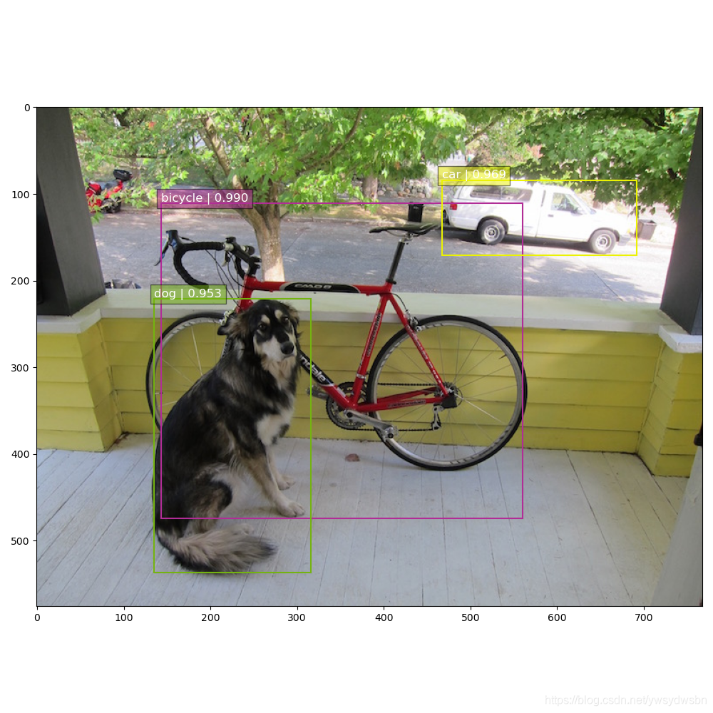
这样检测出来的结果不是很直观。我们最想要的结果应该是在显示框上可以明确显示物体的分类情况。如下图所示:
因此我们需要对SSD-Tensorflow/notebooks/visualization.py进行相应的修改。
修改结果如下:visualization.py
需要修改的地方我都用#================================进行了标注,大家可以对照的看一下。
# Copyright 2017 Paul Balanca. All Rights Reserved.
#
# Licensed under the Apache License, Version 2.0 (the "License");
# you may not use this file except in compliance with the License.
# You may obtain a copy of the License at
#
#     http://www.apache.org/licenses/LICENSE-2.0
#
# Unless required by applicable law or agreed to in writing, software
# distributed under the License is distributed on an "AS IS" BASIS,
# WITHOUT WARRANTIES OR CONDITIONS OF ANY KIND, either express or implied.
# See the License for the specific language governing permissions and
# limitations under the License.
# ==============================================================================
import cv2,sys
import random

import matplotlib.pyplot as plt
import matplotlib.image as mpimg
import matplotlib.cm as mpcm


# =========================================================================== #
# Some colormaps.
# =========================================================================== #
def colors_subselect(colors, num_classes=21):
    dt = len(colors) // num_classes
    sub_colors = []
    for i in range(num_classes):
        color = colors[i*dt]
        if isinstance(color[0], float):
            sub_colors.append([int(c * 255) for c in color])
        else:
            sub_colors.append([c for c in color])
    return sub_colors

colors_plasma = colors_subselect(mpcm.plasma.colors, num_classes=21)
colors_tableau = [(255, 255, 255), (31, 119, 180), (174, 199, 232), (255, 127, 14), (255, 187, 120),
                  (44, 160, 44), (152, 223, 138), (214, 39, 40), (255, 152, 150),
                  (148, 103, 189), (197, 176, 213), (140, 86, 75), (196, 156, 148),
                  (227, 119, 194), (247, 182, 210), (127, 127, 127), (199, 199, 199),
                  (188, 189, 34), (219, 219, 141), (23, 190, 207), (158, 218, 229)]


# =========================================================================== #
# OpenCV drawing.
# =========================================================================== #
def draw_lines(img, lines, color=[255, 0, 0], thickness=2):
    """Draw a collection of lines on an image.
    """
    for line in lines:
        for x1, y1, x2, y2 in line:
            cv2.line(img, (x1, y1), (x2, y2), color, thickness)


def draw_rectangle(img, p1, p2, color=[255, 0, 0], thickness=2):
    cv2.rectangle(img, p1[::-1], p2[::-1], color, thickness)


def draw_bbox(img, bbox, shape, label, color=[255, 0, 0], thickness=2):
    p1 = (int(bbox[0] * shape[0]), int(bbox[1] * shape[1]))
    p2 = (int(bbox[2] * shape[0]), int(bbox[3] * shape[1]))
    cv2.rectangle(img, p1[::-1], p2[::-1], color, thickness)
    p1 = (p1[0]+15, p1[1])
    cv2.putText(img, str(label), p1[::-1], cv2.FONT_HERSHEY_DUPLEX, 0.5, color, 1)


def bboxes_draw_on_img(img, classes, scores, bboxes, colors, thickness=2):
    shape = img.shape
    for i in range(bboxes.shape[0]):
        bbox = bboxes[i]
        color = colors[classes[i]]
        # Draw bounding box...
        p1 = (int(bbox[0] * shape[0]), int(bbox[1] * shape[1]))
        p2 = (int(bbox[2] * shape[0]), int(bbox[3] * shape[1]))
        cv2.rectangle(img, p1[::-1], p2[::-1], color, thickness)
        # Draw text...
        s = '%s/%.3f' % (classes[i], scores[i])
        p1 = (p1[0]-5, p1[1])
        cv2.putText(img, s, p1[::-1], cv2.FONT_HERSHEY_DUPLEX, 0.4, color, 1)


# =========================================================================== #
# Matplotlib show...
# =========================================================================== #
def plt_bboxes(img, classes, scores, bboxes, figsize=(10,10), linewidth=1.5):
    """Visualize bounding boxes. Largely inspired by SSD-MXNET!
    """

    # =========================================
    def num2class(n):
        sys.path.append('../')
        from datasets import pascalvoc_2007 as pas
        x = pas.pascalvoc_common.VOC_LABELS.items()
        for name, item in x:
            if n in item:
                return name
    # =========================================

    fig = plt.figure(figsize=figsize)
    plt.imshow(img)
    height = img.shape[0]
    width = img.shape[1]
    colors = dict()
    class_names = []  # 用来储存类别名(一张图有可能不只一个类别名)
    for i in range(classes.shape[0]):
        cls_id = int(classes[i])
        if cls_id >= 0:
            score = scores[i]
            if cls_id not in colors:
                colors[cls_id] = (random.random(), random.random(), random.random())
            ymin = int(bboxes[i, 0] * height)
            xmin = int(bboxes[i, 1] * width)
            ymax = int(bboxes[i, 2] * height)
            xmax = int(bboxes[i, 3] * width)
            rect = plt.Rectangle((xmin, ymin), xmax - xmin,
                                 ymax - ymin, fill=False,
                                 edgecolor=colors[cls_id],
                                 linewidth=linewidth)
            plt.gca().add_patch(rect)
            # class_name = str(cls_id)
            # ==================================
            class_name = num2class(cls_id)
            class_names.append(class_name)
            # ==================================

            plt.gca().text(xmin, ymin - 2,
                           '{:s} | {:.3f}'.format(class_name, score),
                           bbox=dict(facecolor=colors[cls_id], alpha=0.5),
                           fontsize=12, color='white')
    plt.show()
    # ==================================
    return class_names
    # ==================================
进行测试;
# 测试图片:
from notebooks import visualization
from preprocessing import ssd_vgg_preprocessing
from nets import ssd_vgg_300, ssd_common, np_methods
import matplotlib.image as mpimg
import matplotlib.pyplot as plt
import os
import math
import random
import numpy as np
import tensorflow as tf
import cv2


slim = tf.contrib.slim


gpu_options = tf.GPUOptions(allow_growth=True)

config = tf.ConfigProto(log_device_placement=False, gpu_options=gpu_options)

isess = tf.InteractiveSession(config=config)


net_shape = (300, 300)

data_format = 'NHWC'
# DATA_FORMAT = 'NCHW'  # gpu
# DATA_FORMAT = 'NHWC'  # cpu

img_input = tf.placeholder(tf.uint8, shape=(None, None, 3))


image_pre, labels_pre, bboxes_pre, bbox_img = ssd_vgg_preprocessing.preprocess_for_eval(

    img_input, None, None, net_shape, data_format, resize=ssd_vgg_preprocessing.Resize.WARP_RESIZE)

image_4d = tf.expand_dims(image_pre, 0)


reuse = True if 'ssd_net' in locals() else None

ssd_net = ssd_vgg_300.SSDNet()

with slim.arg_scope(ssd_net.arg_scope(data_format=data_format)):

    predictions, localisations, _, _ = ssd_net.net(
        image_4d, is_training=False, reuse=reuse)


ckpt_filename = './checkpoints/ssd_300_vgg.ckpt'


isess.run(tf.global_variables_initializer())

saver = tf.train.Saver()

saver.restore(isess, ckpt_filename)


ssd_anchors = ssd_net.anchors(net_shape)


def process_image(img, select_threshold=0.5, nms_threshold=.45, net_shape=(300, 300)):

    rimg, rpredictions, rlocalisations, rbbox_img = isess.run([image_4d, predictions, localisations, bbox_img],
                                                              feed_dict={img_input: img})

    rclasses, rscores, rbboxes = np_methods.ssd_bboxes_select(
        rpredictions, rlocalisations, ssd_anchors,
        select_threshold=select_threshold, img_shape=net_shape, num_classes=21, decode=True)
    rbboxes = np_methods.bboxes_clip(rbbox_img, rbboxes)

    rclasses, rscores, rbboxes = np_methods.bboxes_sort(
        rclasses, rscores, rbboxes, top_k=400)

    rclasses, rscores, rbboxes = np_methods.bboxes_nms(
        rclasses, rscores, rbboxes, nms_threshold=nms_threshold)

    rbboxes = np_methods.bboxes_resize(rbbox_img, rbboxes)

    return rclasses, rscores, rbboxes


image_path = './demo/dog.jpg'  # 图片路径

img = mpimg.imread(image_path)

rclasses, rscores, rbboxes = process_image(img)  # 这里传入图片

# labeled_img = visualization.bboxes_draw_on_img(
#     img, rclasses, rscores, rbboxes, visualization.colors_plasma)  # 返回标注图片

visualization.plt_bboxes(img, rclasses, rscores, rbboxes)  # 展示(plt)标注图片
显示框明确显示物体的分类:

