在实际项目中,我们往往需要对特定的数据进行分类,那么首先就需要根据需求制作数据集了。接下来我将以自己之前做的一个手势识别分类项目为例子,详细讲解制作图片数据集的具体操作过程。
1. 数据预处理
1.1 数据准备
在项目中,需要进行12种手势的分类。那么首先需要收集每一种类的图片(10张以上)到每个类别的文件夹中,文件夹以手势类别命名,图片不用命名。

1.2 数据增强
如果我们只用上面12个文件夹里面的120张图片数据,是无法训练出模型的,会使得模型过拟合,因此只能祭出 data augmentation(数据增强)神器了,通过旋转,平移,拉伸 等操作每张图片生成150张,这样图片就变成了18000张。下面是 data augmentation 的代码:
在深度学习中,我们经常需要用到一些技巧(比如将图片进行旋转,翻转等)来进行data augmentation, 来减少过拟合。 这里,我们主要用到的是深度学习框架keras中的ImageDataGenerator进行data augmentation。
datagen = ImageDataGenerator(
        rotation_range=40,
        width_shift_range=0.2,
        height_shift_range=0.2,
        rescale=1./255,
        shear_range=0.2,
        zoom_range=0.2,
        horizontal_flip=True,
        fill_mode='nearest',
        cval=0,
        channel_shift_range=0,
        horizontal_flip=False,
        vertical_flip=False,
        rescale=None)
参数
- rotation_range:整数,数据提升时图片随机转动的角度
- width_shift_range:浮点数,图片宽度的某个比例,数据提升时图片水平偏移的幅度`
- height_shift_range:浮点数,图片高度的某个比例,数据提升时图片竖直偏移的幅度 rescale:
- 重放缩因子,默认为None. 如果为None或0则不进行放缩,否则会将该数值乘到数据上(在应用其他变换之前)
- shear_range:浮点数,剪切强度(逆时针方向的剪切变换角度)
- zoom_range:浮点数或形如[lower,upper]的列表,随机缩放的幅度,若为浮点数,则相当于[lower,upper] =
[1 - zoom_range, 1+zoom_range] - fill_mode:‘constant’,‘nearest’,‘reflect’或‘wrap’之一,当进行变换时超出边界的点将根据本参数给定的方法进行处理
- cval:浮点数或整数,当fill_mode=constant时,指定要向超出边界的点填充的值
- channel_shift_range: Float. Range for random channel shifts.
- horizontal_flip:布尔值,进行随机水平翻转
- vertical_flip:布尔值,进行随机竖直翻转 rescale: 重放缩因子,默认为None.
如果为None或0则不进行放缩,否则会将该数值乘到数据上.
2. TensorFlow读取数据的三种方式
在讲述在TensorFlow上的数据读取方式之前,有必要了解一下TensorFlow的系统架构,如下图所示:

TensorFlow的系统架构分为两个部分:
① 前端系统:提供编程模型,负责构造计算图;
② 后端系统:提供运行时环境,负责执行计算图。
在处理数据的过程当中,由于现在的硬件性能的极大提升,数值计算过程可以通过加强硬件的方式来改善,因此数据读取(即IO)往往会成为系统运行性能的瓶颈。在TensorFlow框架中提供了三种数据读取方式:
- Preloaded data: 预加载数据
- Feeding: placeholder, feed_dict由占位符代替数据,运行时填入数据
- Reading from file: 从文件中直接读取
以上三种读取方式各有自己的特点,在了解这些特点或区别之前,需要知道TensorFlow是如何进行工作的。
TF的核心是用C++写的,这样的好处是运行快,缺点是调用不灵活。而Python恰好相反,所以结合两种语言的优势。涉及计算的核心算子和运行框架是用C++写的,并提供API给Python。Python调用这些API,设计训练模型(Graph),再将设计好的Graph给后端去执行。简而言之,Python的角色是Design,C++是Run。
1.1 Preload data: constant 预加载数据
特点:数据直接嵌入graph, 由graph传入session中运行
import tensorflow as tf

#设计graph
x = tf.constant([1,2,3], name='x')
y = tf.constant([2,3,4], name='y')
z = tf.add(x,y, name='z')

#打开一个session,计算z
with tf.Session() as sess:
    print(sess.run(z))


#运行结果如下:
#[3 5 7]
在设计Graph的时候,x和y就被定义成了两个有值的列表,在计算z的时候直接取x和y的值。
1.2 Feeding: placeholder, feed_dict
特点:由占位符代替数据,运行时填入数据
import tensorflow as tf

#设计graph,用占位符代替
x = tf.placeholder(tf.int16)
y = tf.placeholder(tf.int16)
z = tf.add(x,y, name='z')

#打开一个session
with tf.Session() as sess:
    #创建数据
    xs = [1,2,3]
    ys = [2,3,4]
    #运行session,用feed_dict来将创建的数据传递进占位符
    print(sess.run(z, feed_dict={x: xs, y: ys}))
#运行结果如下:
#[3 5 7]
1.3 Reading From File:直接从文件中读取
前两种方法很方便,但是遇到大型数据的时候就会很吃力,即使是Feeding,中间环节的增加也是不小的开销,比如数据类型转换等等。最优的方案就是在Graph定义好文件读取的方法,让TF自己去从文件中读取数据,并解码成可使用的样本集。
我们可以使用QueueRunner和Coordinator来实现bin文件,以及csv文件、TFRecord格式文件的读取,不过这里我们采用隐式创建线程的方法。在讲解具体代码之前,我们需要先来讲解关于TensorFlow中的队列机制和线程。
3. 队列和线程
直接从文件中读取数据的方式,需要设计成队列(Queue)的方式才能较好的解决IO瓶颈的问题,同时需要使用多线程来提高图片的批获取效率。
TensorFlow提供了多线程队列存取机制,主要涉及三个概念:Queue、QueueRunner及Coordinator.
3.1 队列(Queue)
队列是常用的数据结构之一,TensorFlow在各个设备(CPU、GPU、磁盘等)之间传递数据时使用了队列。例如,在CPU与GPU之间传递数据是非常缓慢的,为了避免数据传递带来的耗时瓶颈问题,采用异步的方式,CPU不断往队列传入数据,GPU不断从队列中读取数据。
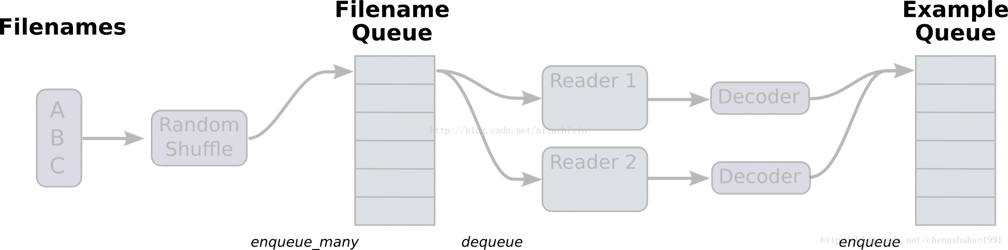
在上图中,首先由一个单线程把文件名堆入队列,两个Reader同时从队列中取文件名并读取数据,Decoder将读出的数据解码后堆入样本队列,最后单个或批量取出样本(图中没有展示样本出列)。我们这里通过三段代码逐步实现上图的数据流,这里我们不使用随机,让结果更清晰。
-
队列数据读取机制:
tf.train.string_input_producer()
tf.train.start_queue_runners() -
文件队列,通过tf.train.string_input_producer()函数来创建,文件名队列不包含文件的具体内容,只是在队列中记录所有的文件名,所以可以在这个函数中对文件设置多个epoch,并对其进行shuffle。这个函数只是创建一个文件队列,并指定入队的操作由几个线程同时完成。真正的读取文件名内容是从执行了tf.train.start_queue_runners()开始的,start_queue_runners返回一个op,一旦执行这个op,文件名队列就开始被填充了。
-
内存队列,这个队列不需要用户手动创建,有了文件名队列后,start_queue_runners之后,Tensorflow会自己维护内存队列并保证用户时时有数据可读。
-
详细内容请看这篇文章
3.2线程(Coordinator)
Coordinator用于管理线程,如管理线程同步等操作。
#创建一个协调器,管理线程
coord = tf.train.Coordinator()
#启动QueueRunner, 此时文件名才开始进队。
threads=tf.train.start_queue_runners(sess=sess,coord=coord)
.....
#关闭线程协调器
coord.request_stop()
coord.join(threads)
4. 异常处理
通过queue runners启动的线程不仅仅只处理推送样本到队列。他们还捕捉和处理由队列产生的异常,包括OutOfRangeError异常,这个异常是用于报告队列被关闭。 使用Coordinator对象的训练程序在主循环中必须同时捕捉和报告异常。 下面是对上面训练循环的改进版本。
try:
    for step in xrange(1000000):
        if coord.should_stop():
            break
        sess.run(train_op)
except Exception, e:
   # Report exceptions to the coordinator.
   coord.request_stop(e)

# Terminate as usual.  It is innocuous to request stop twice.
coord.request_stop()
coord.join(threads)
5. 生成和读取TFRecords文件
那么接下来就是要将图片数据生成文件格式了,我们这里采用的是TFRecord格式。
-
TensorFlow提供了TFRecords的格式来统一存储数据,理论上,TFRecords可以存储任何形式的数据。
-
TFRecords是一种二进制文件,可先将图片和标签制作成该格式的文件。使用TFRecords进行数据读取,会提高内存利用率。
-
用 tf.train.Example的协议存储训练数据。训练数据的特征用键值对的形式表示。如:‘img_raw’:值 ‘label’:值,值是Byteslist/FloatList/int64List
-
用SerializeToString()把数据序列化成字符串存储。
5.1 生成TFRecords文件
writer = tf.python_io.TFRecordWriter(tfRecordName)#新建一个writer

for 循环遍历每张图和标签:
   example = tf.train.Example(features=tf.train.Features(feature={
       'img_raw': tf.train.Feature(bytes_list=tf.train.BytesList(value=[img_raw])),
       'label': tf.train.Feature(int64_list=tf.train.Int64List(value=labels))
   }))#把每张图片和标签封装到example中,feature为字典形式
   writer.write(example.SerializeToString())#把example进行序列化
writer.close()
5.2 读取TFRecords文件
filename_queue = tf.train.string_input_producer([tfRecord_path])
reader = tf.TFRecordReader()#新建一个reader
_, serialized_example = reader.read(filename_queue)
features = tf.parse_single_example(serialized_example,
            features={
                'label': tf.FixedLenFeature([n_class], tf.int64),
                'img_raw': tf.FixedLenFeature([], tf.string)
            })#解序列化
img = tf.decode_raw(features['img_raw'], tf.uint8)#恢复img_raw到img
img.set_shape([img_height*img_width])#把img的形状变成一行784列
img = tf.cast(img, tf.float32) * (1. / 255)#把img的每个元素变成0-1之间的浮点数
label = tf.cast(features['label'], tf.float32)#把label的每个元素变成浮点数
完整代码
from keras.preprocessing.image import ImageDataGenerator, img_to_array, load_img
import os
import time

datagen = ImageDataGenerator(
    rotation_range=20,
    width_shift_range=0.15,
    height_shift_range=0.15,
    zoom_range=0.15,
    shear_range=0.2,
    horizontal_flip=True,
	fill_mode='nearest')

print("start.....: " + str((time.strftime('%Y-%m-%d %H:%M:%S'))))


dirs = os.listdir("D:/360MoveData/Users/ASUS/Desktop/gesture/音量减")
for filename in dirs:
    img = load_img("D:/360MoveData/Users/ASUS/Desktop/gesture/音量减/{}".format(filename))
    x = img_to_array(img)
    # print(x.shape)
    x = x.reshape((1,) + x.shape) #datagen.flow要求rank为4
    # print(x.shape)
    datagen.fit(x)
    prefix = filename.split('.')[0]
    print(prefix)
    counter = 0
    for batch in datagen.flow(x, batch_size=4 , save_to_dir='D:/360MoveData/Users/ASUS/Desktop/gesture_data/音量减', save_prefix=prefix, save_format='jpg'):
        counter += 1
        if counter > 150:
            break  # 否则生成器会退出循环

print("end....: " + str((time.strftime('%Y-%m-%d %H:%M:%S'))))
import os
import numpy as np
from PIL import Image
import tensorflow as tf


W = 100  # 图片原来的长度
H = 100  # 图片原来的高度
Channels = 3  # 图片原来的通道数
n_classes=12

def get_files(file_dir, ratio=0.8):
    """得到训练集和验证集的图像列表和标签列表,默认划分比例为0.8"""
    one = []
    label_one = []
    two = []
    label_two = []
    seven = []
    label_seven = []
    nine = []
    label_nine = []
    call= []
    label_call = []
    good = []
    label_good = []
    home = []
    label_home = []
    rock = []
    label_rock = []
    shangyishou = []
    label_shangyishou = []
    xiayishou = []
    label_xiayishou = []
    yinliangjia = []
    label_yinliangjia = []
    yinliangjian = []
    label_yinliangjian = []
    for file in os.listdir(file_dir):
        pp = os.path.join(file_dir, file)
        for pic in os.listdir(pp):
            pic_path = os.path.join(pp, pic)
            if file == "1":
                one.append(pic_path)  # 读取所在位置名称
                label_one.append(0)  # labels标签为0
            elif file == "2":
                two.append(pic_path)  # 读取所在位置名称
                label_two.append(1)  # labels标签为1
            elif file == "7":
                seven.append(pic_path)  # 读取所在位置名称
                label_seven.append(2)  # labels标签为2
            elif file == "9":
                nine.append(pic_path)  # 读取所在位置名称
                label_nine.append(3)  # labels标签为3
            elif file == "call":
                call.append(pic_path)  # 读取所在位置名称
                label_call.append(4)  # labels标签为4
            elif file == "good":
                good.append(pic_path)  # 读取所在位置名称
                label_good.append(5)  # labels标签为5
            elif file == "home":
                home.append(pic_path)  # 读取所在位置名称
                label_home.append(6)  # labels标签为6
            elif file == "rock":
                rock.append(pic_path)  # 读取所在位置名称
                label_rock.append(7)  # labels标签为7
            elif file == "上一首":
                shangyishou.append(pic_path)  # 读取所在位置名称
                label_shangyishou.append(8)  # labels标签为8
            elif file == "下一首":
                xiayishou.append(pic_path)  # 读取所在位置名称
                label_xiayishou.append(9)  # labels标签为9
            elif file == "音量加":
                yinliangjia.append(pic_path)  # 读取所在位置名称
                label_yinliangjia.append(10)  # labels标签为10
            elif file == "音量减":
                yinliangjian.append(pic_path)  # 读取所在位置名称
                label_yinliangjian.append(11)  # labels标签为11

    # 对多维数组进行打乱排列时,默认是对第一个维度也就是列维度进行随机打乱
    np.random.shuffle(one)
    np.random.shuffle(two)
    np.random.shuffle(seven)
    np.random.shuffle(nine)
    np.random.shuffle(call)
    np.random.shuffle(good)
    np.random.shuffle(home)
    np.random.shuffle(rock)
    np.random.shuffle(shangyishou)
    np.random.shuffle(xiayishou)
    np.random.shuffle(yinliangjia)
    np.random.shuffle(yinliangjian)

    # 按比例划分训练集和验证集
    s0 = np.int(len(one) * ratio)  # 799 * 0.8 = 639.2
    s1 = np.int(len(two) * ratio)  # 633 * 0.8 = 506.4
    s2 = np.int(len(seven) * ratio)  # 898 * 0.8 = 718.4
    s3 = np.int(len(nine) * ratio)  # 641 * 0.8 = 512.8
    s4 = np.int(len(call) * ratio)  # 699 * 0.8 = 559.2
    s5 = np.int(len(good) * ratio)  # 799 * 0.8 = 639.2
    s6 = np.int(len(home) * ratio)  # 633 * 0.8 = 506.4
    s7 = np.int(len(rock) * ratio)  # 898 * 0.8 = 718.4
    s8 = np.int(len(shangyishou) * ratio)  # 641 * 0.8 = 512.8
    s9 = np.int(len(xiayishou) * ratio)  # 699 * 0.8 = 559.2
    s10 = np.int(len(yinliangjia) * ratio)  # 799 * 0.8 = 639.2
    s11 = np.int(len(yinliangjian) * ratio)  # 699 * 0.8 = 559.2


    # np.hstack():在水平方向上平铺;np.vstack():在竖直方向上堆叠
    # 506 + 718 + 515 + 559 + 639 = 2934
    # 633 + 898 + 641 + 699 + 799 - 736
    tra_image_list = np.hstack(
        (one[:s0], two[:s1], seven[:s2], nine[:s3], call[:s4],good[:s5],
         home[:s6], rock[:s7], shangyishou[:s8], xiayishou[:s9], yinliangjia[:s10],yinliangjian[:s11]))
    tra_label_list = np.hstack(
        (label_one[:s0], label_two[:s1], label_seven[:s2], label_nine[:s3], label_call[:s4],label_good[:s5],
         label_home[:s6], label_rock[:s7], label_shangyishou[:s8], label_xiayishou[:s9], label_yinliangjia[:s10],label_yinliangjian[:s11]))
    val_image_list = np.hstack(
        (one[s0:], two[s1:], seven[s2:], nine[s3:], call[s4:], good[s5:],
        home[s6:], rock[s7:], shangyishou[s8:], xiayishou[s9:], yinliangjia[s10:], yinliangjian[s11:]))  # 1行736列
    val_label_list = np.hstack(
        (label_one[s0:], label_two[s1:], label_seven[s2:], label_nine[s3:], label_call[s4:], label_good[s5:],
        label_home[s6:], label_rock[s7:], label_shangyishou[s8:], label_xiayishou[s9:], label_yinliangjia[s10:], label_yinliangjian[s11:]))  # 1行736列

    print("There are %d tra_image_list \nThere are %d tra_label_list \n"
          "There are %d val_image_list \nThere are %d val_label_list \n"
          % (len(tra_image_list), len(tra_label_list), len(val_image_list),
             len(val_label_list)))

    # 2行2934列,第一行是图像列表,第二行时标签列表
    tra_temp = np.array([tra_image_list, tra_label_list])
    # 2行736列,第一行是图像列表,第二行时标签列表
    val_temp = np.array([val_image_list, val_label_list])

    # 对于二维 ndarray,transpose在不指定参数是默认是矩阵转置。对于一维的shape,转置是不起作用的.
    tra_temp = tra_temp.transpose()  # 转置后变成2934行2列,第一列为图像列表,第二列为标签列表
    val_temp = val_temp.transpose()  # 转置后变成736行2列,第一列为图像列表,第二列为标签列表

    # 对多维数组进行打乱排列时,默认是对第一个维度也就是列维度进行随机打乱
    np.random.shuffle(tra_temp)  # 随机排列,注意调试时不用
    np.random.shuffle(val_temp)

    tra_image_list = list(tra_temp[:, 0])
    tra_label_list = list(tra_temp[:, 1])
    tra_label_list = [int(i) for i in tra_label_list]
    val_image_list = list(val_temp[:, 0])
    val_label_list = list(val_temp[:, 1])
    val_label_list = [int(i) for i in val_label_list]

    # 注意,image_list里面其实存的图片文件的路径
    return tra_image_list, tra_label_list, val_image_list, val_label_list


def image2tfrecord(image_list, label_list, filename):
    # 生成字符串型的属性
    def _bytes_feature(value):
        return tf.train.Feature(bytes_list=tf.train.BytesList(value=[value]))

    # 生成整数型的属性
    def _int64_feature(value):
        return tf.train.Feature(int64_list=tf.train.Int64List(value=[value]))

    len2 = len(image_list)
    print("len=", len2)
    # 创建一个writer来写TFRecord文件,filename是输出TFRecord文件的地址
    writer = tf.python_io.TFRecordWriter(filename)

    for i in range(len2):
        print(i)
        # 读取图片并解码
        image = Image.open(image_list[i])
        image = image.resize((100, 100))
        # 转化为原始字节(tostring()已经被移除,用tobytes()替代)
        image_bytes = image.tobytes()
        # 创建字典
        features = {}
        # 用bytes来存储image
        features['image_raw'] = _bytes_feature(image_bytes)
        # 用int64来表达label
        features['label'] = _int64_feature(label_list[i])
        # 将所有的feature合成features
        tf_features = tf.train.Features(feature=features)
        # 将样本转成Example Protocol Buffer,并将所有的信息写入这个数据结构
        tf_example = tf.train.Example(features=tf_features)
        # 序列化样本
        tf_serialized = tf_example.SerializeToString()
        # 将序列化的样本写入trfrecord
        writer.write(tf_serialized)
    writer.close()

def get_batch(tfrecords_file, batch_size):
    '''阅读和解码TFRecord文件,生成(image, label) 批数据
    参数:
        tfrecords_file: TFRecord文件的目录
        batch_size: 批数据的大小
    返回:
        image_batch: 4维张量 - [batch_size, height, width, channel]
        label_batch: 2维张量 - [batch_size, n_classes]
    '''
    # tf.train.string_input_producer函数会使用初始化时提供的文件列表创建一个输入队列
    # 输入队列中原始的元素为文件列表中的所有文件,可以设置shuffle参数。
    filename_queue = tf.train.string_input_producer([tfrecords_file])
    # 创建一个reader来读取TFRecord文件中的样例
    reader = tf.TFRecordReader()
    # 从文件中读出一个样例。也可以使用read_up_to函数一次性读取多个案例
    _, serialized_example = reader.read(filename_queue)  # 返回文件名和文件
    # 解析读入的一个样例。如果需要解析多个样例,可以用parse_example函数
    img_features = tf.parse_single_example(
        serialized_example,
        features={
            # tf.FixedLenFeature解析的结果为一个tensor
            'label': tf.FixedLenFeature([], tf.int64),
            'image_raw': tf.FixedLenFeature([], tf.string),
        })  # 取出包含image和label的feature对象

    # tf.decode_raw可以将字符串解析成图像对应的像素数组
    image = tf.decode_raw(img_features['image_raw'], tf.uint8)
    # 根据图像尺寸,还原图像
    image = tf.reshape(image, [H, W, Channels])
    # 将image的数据格式转换成实数型,并进行归一化处理
    # image = image.astype('float32');image /= 255
    image = tf.cast(image, tf.float32) * (1.0 / 255)
    # 图像标准化是将数据通过去均值实现中心化的处理,更容易取得训练之后的泛化效果
    # 线性缩放image以具有零均值和单位范数。操作计算(x - mean) / adjusted_stddev
    # image = tf.image.per_image_standardization(image)

    # 如果使用其他数据集,需要更改图像大小
    label = tf.cast(img_features['label'], tf.int32)
    # 将多个输入样例组织成一个batch可以提高模型训练的效率
    # 一般image和label分别代表训练样本和这个样本对应的正确标签。
    # batch_size:一个batch中样例的个数
    # num_threads:指定多个线程同时执行入队操作
    # capacity:组合样例的队列中最多可以存储的样例个数。太大,需要占用很多内存资源
    # 太小,出队操作可能会因为没有数据而被阻碍,从而导致训练效率降低。
    image_batch, label_batch = tf.train.batch([image, label],
                                              batch_size=batch_size,
                                              num_threads=4,
                                              capacity=2000)
    # 将类别向量(0~n_classes的整数向量)映射为二值类别矩阵,相当于用one-hot重新编码
    label_batch = tf.one_hot(label_batch, depth=n_classes)
    label_batch = tf.cast(label_batch, dtype=tf.int32)
    label_batch = tf.reshape(label_batch, [batch_size, n_classes])
    # 张量保存的是计算过程。一个张量主要保存了三个属性:name、shape、dtype
    print(label_batch)
    return image_batch, label_batch


if __name__ == "__main__":

    tra_data_dir = './data/gesture_train.tfrecords'
    val_data_dir ='./data/gesture_test.tfrecords'
    path = 'D:/360MoveData/Users/ASUS/Desktop/datasets/'
    tra_img_list, tra_label_list, val_image_list, val_label_list = get_files(path)
    image2tfrecord(tra_img_list, tra_label_list, tra_data_dir)
    image2tfrecord(val_image_list, val_label_list, val_data_dir)
import tensorflow as tf
from tensorflow.python.framework import graph_util
import matplotlib.pyplot as plt
from input_data import get_batch
import os

tra_data_dir = './data/gesture_train.tfrecords'
val_data_dir ='./data/gesture_test.tfrecords'

W = 100  # 图片原来的长度
H = 100  # 图片原来的高度
Channels = 3  # 图片原来的通道数

batch_size = 20  # 定义组合数据batch的大小
num_epochs = 60000  # 训练轮数
n_classes = 12  # 类别数

pb_file_path = "./gesture_model.pb"
MODEL_SAVE_PATH="./model/"
MODEL_NAME="gesture_model"
regularizer = tf.contrib.layers.l2_regularizer(0.0001)
dropout=0.8

"""构造卷积神经网络"""
# 定义两个placeholder,用于输入数据
x = tf.placeholder(tf.float32, shape=[None, H, W, Channels],
                   name="input_x")  ####这个名称很重要!!!
y = tf.placeholder(tf.int32, shape=[None, n_classes], name="input_y")
keep_prob = tf.placeholder(tf.float32, name='keep_prob')
global_step = tf.Variable(0, trainable=False)

with tf.variable_scope('layer1-conv1'):
    conv1_weights = tf.get_variable(
        "weight", [5, 5, 3, 32],
        initializer=tf.truncated_normal_initializer(stddev=0.1))
    conv1_biases = tf.get_variable(
        "bias", [32], initializer=tf.constant_initializer(0.0))
    conv1 = tf.nn.conv2d(
        x, conv1_weights, strides=[1, 1, 1, 1], padding='SAME')
    relu1 = tf.nn.relu(tf.nn.bias_add(conv1, conv1_biases))

with tf.name_scope("layer2-pool1"):
    pool1 = tf.nn.max_pool(
        relu1, ksize=[1, 2, 2, 1], strides=[1, 2, 2, 1], padding="VALID")

with tf.variable_scope("layer3-conv2"):
    conv2_weights = tf.get_variable(
        "weight", [5, 5, 32, 64],
        initializer=tf.truncated_normal_initializer(stddev=0.1))
    conv2_biases = tf.get_variable(
        "bias", [64], initializer=tf.constant_initializer(0.0))
    conv2 = tf.nn.conv2d(
        pool1, conv2_weights, strides=[1, 1, 1, 1], padding='SAME')
    relu2 = tf.nn.relu(tf.nn.bias_add(conv2, conv2_biases))

with tf.name_scope("layer4-pool2"):
    pool2 = tf.nn.max_pool(
        relu2, ksize=[1, 2, 2, 1], strides=[1, 2, 2, 1],
        padding='VALID')

with tf.variable_scope("layer5-conv3"):
    conv3_weights = tf.get_variable(
        "weight", [3, 3, 64, 128],
        initializer=tf.truncated_normal_initializer(stddev=0.1))
    conv3_biases = tf.get_variable(
        "bias", [128], initializer=tf.constant_initializer(0.0))
    conv3 = tf.nn.conv2d(
        pool2, conv3_weights, strides=[1, 1, 1, 1], padding='SAME')
    relu3 = tf.nn.relu(tf.nn.bias_add(conv3, conv3_biases))

with tf.name_scope("layer6-pool3"):
    pool3 = tf.nn.max_pool(
        relu3, ksize=[1, 2, 2, 1], strides=[1, 2, 2, 1],
        padding='VALID')

with tf.variable_scope("layer7-conv4"):
    conv4_weights = tf.get_variable(
        "weight", [3, 3, 128, 128],
        initializer=tf.truncated_normal_initializer(stddev=0.1))
    conv4_biases = tf.get_variable(
        "bias", [128], initializer=tf.constant_initializer(0.0))
    conv4 = tf.nn.conv2d(pool3, conv4_weights, strides=[1, 1, 1, 1],
                         padding='SAME')
    relu4 = tf.nn.relu(tf.nn.bias_add(conv4, conv4_biases))

with tf.name_scope("layer8-pool4"):
    pool4 = tf.nn.max_pool(relu4, ksize=[1, 2, 2, 1],
                           strides=[1, 2, 2, 1], padding='VALID')
    nodes = 6 * 6 * 128
    reshaped = tf.reshape(pool4, [-1, nodes])

with tf.variable_scope('layer9-fc1'):
    fc1_weights = tf.get_variable(
        "weight", [nodes, 1024],
        initializer=tf.truncated_normal_initializer(stddev=0.1))
    if regularizer != None:
        tf.add_to_collection('losses', regularizer(fc1_weights))
    fc1_biases = tf.get_variable(
        "bias", [1024], initializer=tf.constant_initializer(0.1))
    fc1 = tf.nn.relu(tf.matmul(reshaped, fc1_weights) + fc1_biases)
    fc1 = tf.nn.dropout(fc1, keep_prob=keep_prob)

with tf.variable_scope('layer10-fc2'):
    fc2_weights = tf.get_variable(
        "weight", [1024, 512],
        initializer=tf.truncated_normal_initializer(stddev=0.1))
    if regularizer != None:
        tf.add_to_collection('losses', regularizer(fc2_weights))
    fc2_biases = tf.get_variable("bias", [512], initializer=tf.constant_initializer(0.1))

    fc2 = tf.nn.relu(tf.matmul(fc1, fc2_weights) + fc2_biases)
    fc2 = tf.nn.dropout(fc2, keep_prob=keep_prob)

with tf.variable_scope('layer11-fc3'):
    fc3_weights = tf.get_variable(
        "weight", [512, n_classes],
        initializer=tf.truncated_normal_initializer(stddev=0.1))
    if regularizer != None:
        tf.add_to_collection('losses', regularizer(fc3_weights))
    fc3_biases = tf.get_variable(
        "bias", [n_classes], initializer=tf.constant_initializer(0.1))
    logits =tf.add(tf.matmul(fc2, fc3_weights) , fc3_biases,name='outlayer')


# softmax_cross_entropy_with_logits计算交叉熵(废弃)
# cost = tf.reduce_mean(tf.nn.softmax_cross_entropy_with_logits(logits=finaloutput, labels=y))*1000
# logits是batch×classes的一个矩阵,classes为类别数量
# labels是长batch的一个一维数组。当logits判断图片为某一类时,对应classes的位置为1
cost = tf.reduce_mean(tf.nn.sparse_softmax_cross_entropy_with_logits(
    logits=logits, labels=tf.argmax(y, 1)))
# 定义反向传播算法来优化神经网络中的参数
optimize = tf.train.AdamOptimizer(0.001).minimize(cost, global_step=global_step)

prob = tf.nn.softmax(logits, name="probability")
prediction_labels = tf.argmax(prob, axis=1, name="predict")
read_labels = tf.argmax(y, axis=1)

# 判断两个张量的每一维是否相等,如果相等返回True,否则返回False
correct_prediction = tf.equal(prediction_labels, read_labels)
# 这个运算先将布尔型数值转换为实数型,然后计算平均值。
# 这个平均值就是模型在这一组数据上的正确率。
accuracy = tf.reduce_mean(tf.cast(correct_prediction, tf.float32))


# 训练集批数据
tra_image_batch, tra_label_batch = get_batch(
    tfrecords_file=tra_data_dir, batch_size=batch_size)
# 验证集批数据
val_image_batch, val_label_batch = get_batch(
    tfrecords_file=val_data_dir, batch_size=batch_size)

saver = tf.train.Saver()
with tf.Session() as sess:
    # 变量初始化
    init = tf.global_variables_initializer()
    sess.run(init)

    ckpt = tf.train.get_checkpoint_state(MODEL_SAVE_PATH)
    if ckpt and ckpt.model_checkpoint_path:
        saver.restore(sess, ckpt.model_checkpoint_path)

    # 声明一个tf.train.Coordinator类来协同多个线程
    coord = tf.train.Coordinator()
    # tf.train.start_queue_runners函数默认启动tf.GraphKeys.QUEUE_RUNNERS
    # 集合中所有的QueueRunner
    threads = tf.train.start_queue_runners(sess=sess, coord=coord)

    try:
        for epoch_index in range(num_epochs):
            tra_images, tra_labels = sess.run([tra_image_batch, tra_label_batch])
            # 替你刚刚选取的样本训练神经网络并更新参数
            tra_acc,tra_loss,  _ ,step= sess.run(
                [accuracy, cost, optimize,global_step], feed_dict={
                    x: tra_images,
                    y: tra_labels,
                    keep_prob:dropout
                })


            # 每20轮输出一次在验证数据集上的测试结果
            if epoch_index % 20 == 0:
                # 开始在训练集上计算一下准确率和损失函数
                print("index[%s]".center(50, '-') % step)
                print("Tra: loss:{},,accuracy:{}".format(tra_loss, tra_acc*100))

                # 开始在验证集上计算一下准确率和损失函数
                val_images, val_labels = sess.run([val_image_batch, val_label_batch])
                val_acc,val_loss= sess.run(
                    [accuracy,cost], feed_dict={
                        x: val_images,
                        y: val_labels,
                        keep_prob:dropout
                    })
                print("Val: loss:{},accuracy:{}".format(val_loss,val_acc*100))

            if epoch_index % 50 == 0:
                # 将图中的变量及其取值转化为常量,同时将图中不必要的节点去掉。
                # 如果只关心程序中定义的某些计算时,无关的节点就没必要导出并保存
                saver.save(sess, os.path.join(MODEL_SAVE_PATH, MODEL_NAME), global_step=global_step)
                constant_graph = graph_util.convert_variables_to_constants(
                    sess, sess.graph_def, ["predict"])
                with tf.gfile.FastGFile(pb_file_path, mode='wb') as f:
                    f.write(constant_graph.SerializeToString())

    except tf.errors.OutOfRangeError:  # 当遍历结束时,程序会抛出OutOfRangeError
        print('Done training -- epoch limit reached')
    finally:
        # 调用coord.request_stop()函数来停止所有其他的线程
        coord.request_stop()
    # 等待所有线程退出
    coord.join(threads)
    sess.close()
