直線回帰
ベクトル計算
トレーニングや予測モデルは、我々は多くの場合、複数のデータサンプルおよび使用ベクトル演算を処理します。線形回帰ベクトルの計算式の導入前に、2つのベクトルを追加するための二つの方法を考えてみましょう。
ベクターを追加するため1. Aの方法は、2つの要素のスカラー加算を行うための一つ一つに記載のベクターです。
2.ベクトル和は、2つのベクトルベクトル加算に直接実行されるもう一つの方法。
import torch
import time

# init variable a, b as 1000 dimension vector
n = 1000
a = torch.ones(n)
b = torch.ones(n)
# define a timer class to record time
class Timer(object):
    """Record multiple running times."""
    def __init__(self):
        self.times = []
        self.start()

    def start(self):
        # start the timer
        self.start_time = time.time()

    def stop(self):
        # stop the timer and record time into a list
        self.times.append(time.time() - self.start_time)
        return self.times[-1]

    def avg(self):
        # calculate the average and return
        return sum(self.times)/len(self.times)

    def sum(self):
        # return the sum of recorded time
        return sum(self.times)
まず、要素一つずつによってテストループのために使用される2つのベクトルは、スカラ加算を作ります。
timer = Timer()
c = torch.zeros(n)
for i in range(n):
    c[i] = a[i] + b[i]
'%.5f sec' % timer.stop()
さらに、トーチは、2つのベクトルの直接のベクトル加算を行うために使用されます。
timer.start()
d = a + b
'%.5f sec' % timer.stop()
高速フロント後ろの結果は、計算効率を改善するために、ベクトル演算として使用されるべきです。
ゼロを達成するために、線形回帰モデル
# import packages and modules
%matplotlib inline
import torch
from IPython import display
from matplotlib import pyplot as plt
import numpy as np
import random

print(torch.__version__)
データセット生成
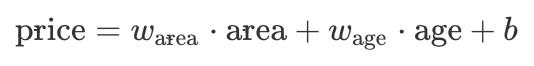
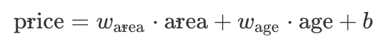
データセットを生成するために線形モデルを使用して、1000個のサンプルのデータセットを生成し、次の線形関係は、データを生成するために使用されます。
# set input feature number
num_inputs = 2
# set example number
num_examples = 1000

# set true weight and bias in order to generate corresponded label
true_w = [2, -3.4]
true_b = 4.2

features = torch.randn(num_examples, num_inputs,
                      dtype=torch.float32)
labels = true_w[0] * features[:, 0] + true_w[1] * features[:, 1] + true_b
labels += torch.tensor(np.random.normal(0, 0.01, size=labels.size()),
                       dtype=torch.float32)
ショーに生成された画像データを用いて、
plt.scatter(features[:, 1].numpy(), labels.numpy(), 1);
データセットを読みます
def data_iter(batch_size, features, labels):
    num_examples = len(features)
    indices = list(range(num_examples))
    random.shuffle(indices)  # random read 10 samples
    for i in range(0, num_examples, batch_size):
        j = torch.LongTensor(indices[i: min(i + batch_size, num_examples)]) # the last time may be not enough for a whole batch
        yield  features.index_select(0, j), labels.index_select(0, j)
batch_size = 10

for X, y in data_iter(batch_size, features, labels):
    print(X, '\n', y)
    break
モデルの初期化パラメータ
w = torch.tensor(np.random.normal(0, 0.01, (num_inputs, 1)), dtype=torch.float32)
b = torch.zeros(1, dtype=torch.float32)

w.requires_grad_(requires_grad=True)
b.requires_grad_(requires_grad=True)
定義モデルの
モデルパラメータを訓練するために使用されるトレーニングの定義:
def linreg(X, w, b):
    return torch.mm(X, w) + b
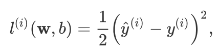
定義の損失関数
、我々は平均二乗誤差損失関数を使用しています:
def squared_loss(y_hat, y):
    return (y_hat - y.view(y_hat.size())) ** 2 / 2
定義された最適化機能
ここでは、少量の確率的勾配降下法で使用される最適化機能であります:

def sgd(params, lr, batch_size):
    for param in params:
        param.data -= lr * param.grad / batch_size # ues .data to operate param without gradient track
トレーニング
時にデータセット、モデル、および関数定義がトレーニングモデルの準備をするために行うことができた後、損失関数を最適化します。
# super parameters init
lr = 0.03
num_epochs = 5

net = linreg
loss = squared_loss

# training
for epoch in range(num_epochs):  # training repeats num_epochs times
    # in each epoch, all the samples in dataset will be used once

    # X is the feature and y is the label of a batch sample
    for X, y in data_iter(batch_size, features, labels):
        l = loss(net(X, w, b), y).sum()
        # calculate the gradient of batch sample loss
        l.backward()
        # using small batch random gradient descent to iter model parameters
        sgd([w, b], lr, batch_size)
        # reset parameter gradient
        w.grad.data.zero_()
        b.grad.data.zero_()
    train_l = loss(net(features, w, b), labels)
    print('epoch %d, loss %f' % (epoch + 1, train_l.mean().item()))
w, true_w, b, true_b
pytorchを達成するために、単純な線形回帰モデルを使用して
import torch
from torch import nn
import numpy as np
torch.manual_seed(1)

print(torch.__version__)
torch.set_default_tensor_type('torch.FloatTensor')
データセットを生成
ゼロベースのデータセットの実現と、ここで生成されたがまったく同じです。
num_inputs = 2
num_examples = 1000

true_w = [2, -3.4]
true_b = 4.2

features = torch.tensor(np.random.normal(0, 1, (num_examples, num_inputs)), dtype=torch.float)
labels = true_w[0] * features[:, 0] + true_w[1] * features[:, 1] + true_b
labels += torch.tensor(np.random.normal(0, 0.01, size=labels.size()), dtype=torch.float)
データセットを読みます
import torch.utils.data as Data

batch_size = 10

# combine featues and labels of dataset
dataset = Data.TensorDataset(features, labels)

# put dataset into DataLoader
data_iter = Data.DataLoader(
    dataset=dataset,            # torch TensorDataset format
    batch_size=batch_size,      # mini batch size
    shuffle=True,               # whether shuffle the data or not
    num_workers=2,              # read data in multithreading
)
for X, y in data_iter:
    print(X, '\n', y)
    break
定義モデル
class LinearNet(nn.Module):
    def __init__(self, n_feature):
        super(LinearNet, self).__init__()      # call father function to init
        self.linear = nn.Linear(n_feature, 1)  # function prototype: `torch.nn.Linear(in_features, out_features, bias=True)`
    def forward(self, x):
        y = self.linear(x)
        return y

net = LinearNet(num_inputs)
print(net)
# ways to init a multilayer network
# method one
net = nn.Sequential(
    nn.Linear(num_inputs, 1)
    # other layers can be added here
    )

# method two
net = nn.Sequential()
net.add_module('linear', nn.Linear(num_inputs, 1))
# net.add_module ......

# method three
from collections import OrderedDict
net = nn.Sequential(OrderedDict([
          ('linear', nn.Linear(num_inputs, 1))
          # ......
        ]))

print(net)
print(net[0])
モデルの初期化パラメータ
from torch.nn import init

init.normal_(net[0].weight, mean=0.0, std=0.01)
init.constant_(net[0].bias, val=0.0)  # or you can use `net[0].bias.data.fill_(0)` to modify it directly
for param in net.parameters():
    print(param)
定義された損失関数
loss = nn.MSELoss()    # nn built-in squared loss function
                       # function prototype: `torch.nn.MSELoss(size_average=None, reduce=None, reduction='mean')`
定義された最適化機能
import torch.optim as optim

optimizer = optim.SGD(net.parameters(), lr=0.03)   # built-in random gradient descent function
print(optimizer)  # function prototype: `torch.optim.SGD(params, lr=, momentum=0, dampening=0, weight_decay=0, nesterov=False)`
トレーニング
num_epochs = 3
for epoch in range(1, num_epochs + 1):
    for X, y in data_iter:
        output = net(X)
        l = loss(output, y.view(-1, 1))
        optimizer.zero_grad() # reset gradient, equal to net.zero_grad()
        l.backward()
        optimizer.step()
    print('epoch %d, loss: %f' % (epoch, l.item()))
# result comparision
dense = net[0]
print(true_w, dense.weight.data)
print(true_b, dense.bias.data)
2つの実装の比較
実現1.ゼロベース(学習のために推奨)
ニューラルネットワークモデルと基本的な原則をよりよく理解
2.シンプルpytorch実装
モデルの設計と実装をより迅速に完了することができます
