ロジスティック回帰
データ
私たちは、学生が大学に入学されているかどうかを予測するロジスティック回帰モデルを構築します。あなたは大学部門の管理者であると仮定し、次の2回の試験の結果に基づいて、入場の各申請者の機会を決定します。あなたはロジスティック回帰のトレーニングセットとして使用することができ、応募者データの以前の歴史を持っています。各トレーニングたとえば、あなたが応募し、入学の意思決定2回の試験のスコアを持っています。これを行うために、我々はテストの点数に基づいて入学の確率を推定するために、分類モデルを確立していきます。
#三大件
import numpy as np
import pandas as pd
import matplotlib.pyplot as plt
%matplotlib inline
import os
path = 'data' + os.sep + 'LogiReg_data.txt'
pdData = pd.read_csv(path, header=None, names=['Exam 1', 'Exam 2', 'Admitted'])
pdData.head()| 試験1 | 試験2 | 入院 | |
|---|---|---|---|
| 0 | 34.623660 | 78.024693 | 0 |
| 1 | 30.286711 | 43.894998 | 0 |
| 2 | 35.847409 | 72.902198 | 0 |
| 3 | 60.182599 | 86.308552 | 1 |
| 4 | 79.032736 | 75.344376 | 1 |
pdData.shape(100, 3)positive = pdData[pdData['Admitted'] == 1] # returns the subset of rows such Admitted = 1, i.e. the set of *positive* examples
negative = pdData[pdData['Admitted'] == 0] # returns the subset of rows such Admitted = 0, i.e. the set of *negative* examples
fig, ax = plt.subplots(figsize=(10,5))
ax.scatter(positive['Exam 1'], positive['Exam 2'], s=30, c='b', marker='o', label='Admitted')
ax.scatter(negative['Exam 1'], negative['Exam 2'], s=30, c='r', marker='x', label='Not Admitted')
ax.legend()
ax.set_xlabel('Exam 1 Score')
ax.set_ylabel('Exam 2 Score')Text(0, 0.5, 'Exam 2 Score')
ロジスティック回帰
目標:分類器の設置(解決三つのパラメータ$ \ theta_0 \ theta_1 \ theta_2 $)
閾値を設定する閾値は、受付結果に応じて決定されます
モジュールを完了するには
sigmoid:確率関数のマッピングmodel:予測結果の値を返します。cost:計算されたパラメータの損失gradient:勾配方向は、各パラメータを算出しますdescent:パラメータの更新accuracy:精度
sigmoid 機能
\ [G(Z)= \ FRAC {1} {1 + E ^ { - }}と\]
def sigmoid(z):
    return 1 / (1 + np.exp(-z))
nums = np.arange(-10, 10, step=1) #creates a vector containing 20 equally spaced values from -10 to 10
fig, ax = plt.subplots(figsize=(12,4))
ax.plot(nums, sigmoid(nums), 'r')[<matplotlib.lines.Line2D at 0x19dbf1cd948>]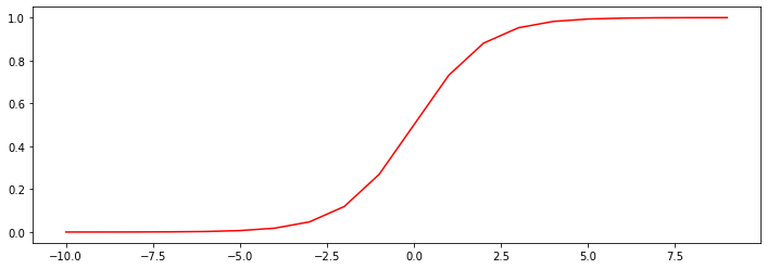
シグモイド
- \(G:\ mathbb {R} \に[0,1] \)
- \(G(0)= 0.5 \)
- \(G( - \ inftyの)= 0 \)
- \(G(+ \ inftyの)= 1 \)
def model(X, theta):

    return sigmoid(np.dot(X, theta.T))
\ [\ {アレイ} {CCC} \開始{pmatrixの} \ theta_ {0}&\ theta_ {1}&\ theta_ {2} \端{pmatrixのを}開始&\回&\ {pmatrixの} 1 \\ X_始まります{1} \\ X_ {2} \端{pmatrixの} \端{アレイ} = \ theta_ {0} + \ theta_ {1} X_ {1} + \ theta_ {2} X_ {2} \]
pdData.insert(0, 'Ones', 1) # in a try / except structure so as not to return an error if the block si executed several times


# set X (training data) and y (target variable)
orig_data = pdData.as_matrix() # convert the Pandas representation of the data to an array useful for further computations
cols = orig_data.shape[1]
X = orig_data[:,0:cols-1]
y = orig_data[:,cols-1:cols]

# convert to numpy arrays and initalize the parameter array theta
#X = np.matrix(X.values)
#y = np.matrix(data.iloc[:,3:4].values) #np.array(y.values)
theta = np.zeros([1, 3])
d:\python\py376\lib\site-packages\ipykernel_launcher.py:5: FutureWarning: Method .as_matrix will be removed in a future version. Use .values instead.
"""X[:5]array([[ 1. , 34.62365962, 78.02469282],
[ 1. , 30.28671077, 43.89499752],
[ 1. , 35.84740877, 72.90219803],
[ 1. , 60.18259939, 86.3085521 ],
[ 1. , 79.03273605, 75.34437644]])y[:5]array([[0.],
[0.],
[0.],
[1.],
[1.]])thetaarray([[0., 0., 0.]])X.shape, y.shape, theta.shape((100, 3), (100, 1), (1, 3))損失関数
マイナスの対数尤度関数
\ [D(H_ \シータ(
X)、Y)= -y \ログ(H_ \シータ(X)) - (1-Y)\ログ(1-H_ \シータ(X))\] の損失を平均
\ [J(\シータ)= \ FRAC {1} {N} \ sum_ {I = 1} ^ {n}はD(H_ \シータ(X_I)、Y_I)\]
def cost(X, y, theta):
    left = np.multiply(-y, np.log(model(X, theta)))
    right = np.multiply(1 - y, np.log(1 - model(X, theta)))
    return np.sum(left - right) / (len(X))
cost(X, y, theta)0.6931471805599453勾配計算
\ [\ FRAC {\部分J} {\部分\ theta_j} = - \ FRAC {1} {M} \ sum_ {i = 1} ^ N(Y_I - H_ \シータ(X_I))X_ {IJ} \]
def gradient(X, y, theta):
    grad = np.zeros(theta.shape)
    error = (model(X, theta)- y).ravel()
    for j in range(len(theta.ravel())): #for each parmeter
        term = np.multiply(error, X[:,j])
        grad[0, j] = np.sum(term) / len(X)

    return grad
勾配降下
異なる方法の3比較勾配降下
STOP_ITER = 0
STOP_COST = 1
STOP_GRAD = 2

def stopCriterion(type, value, threshold):
    #设定三种不同的停止策略
    if type == STOP_ITER:        return value > threshold
    elif type == STOP_COST:      return abs(value[-1]-value[-2]) < threshold
    elif type == STOP_GRAD:      return np.linalg.norm(value) < threshold
import numpy.random
#洗牌
def shuffleData(data):
np.random.shuffle(data)
cols = data.shape[1]
X = data[:, 0:cols-1]
y = data[:, cols-1:]
return X, yimport time
def descent(data, theta, batchSize, stopType, thresh, alpha):
#梯度下降求解
init_time = time.time()
i = 0 # 迭代次数
k = 0 # batch
X, y = shuffleData(data)
grad = np.zeros(theta.shape) # 计算的梯度
costs = [cost(X, y, theta)] # 损失值
while True:
grad = gradient(X[k:k+batchSize], y[k:k+batchSize], theta)
k += batchSize #取batch数量个数据
if k >= n:
k = 0
X, y = shuffleData(data) #重新洗牌
theta = theta - alpha*grad # 参数更新
costs.append(cost(X, y, theta)) # 计算新的损失
i += 1
if stopType == STOP_ITER: value = i
elif stopType == STOP_COST: value = costs
elif stopType == STOP_GRAD: value = grad
if stopCriterion(stopType, value, thresh): break
return theta, i-1, costs, grad, time.time() - init_timedef runExpe(data, theta, batchSize, stopType, thresh, alpha):
#import pdb; pdb.set_trace();
theta, iter, costs, grad, dur = descent(data, theta, batchSize, stopType, thresh, alpha)
name = "Original" if (data[:,1]>2).sum() > 1 else "Scaled"
name += " data - learning rate: {} - ".format(alpha)
if batchSize==n: strDescType = "Gradient"
elif batchSize==1: strDescType = "Stochastic"
else: strDescType = "Mini-batch ({})".format(batchSize)
name += strDescType + " descent - Stop: "
if stopType == STOP_ITER: strStop = "{} iterations".format(thresh)
elif stopType == STOP_COST: strStop = "costs change < {}".format(thresh)
else: strStop = "gradient norm < {}".format(thresh)
name += strStop
print ("***{}\nTheta: {} - Iter: {} - Last cost: {:03.2f} - Duration: {:03.2f}s".format(
name, theta, iter, costs[-1], dur))
fig, ax = plt.subplots(figsize=(12,4))
ax.plot(np.arange(len(costs)), costs, 'r')
ax.set_xlabel('Iterations')
ax.set_ylabel('Cost')
ax.set_title(name.upper() + ' - Error vs. Iteration')
return theta異なるストップ戦略
反復回数を設定します。
#选择的梯度下降方法是基于所有样本的
n=100
runExpe(orig_data, theta, n, STOP_ITER, thresh=5000, alpha=0.000001)
***Original data - learning rate: 1e-06 - Gradient descent - Stop: 5000 iterations
Theta: [[-0.00027127 0.00705232 0.00376711]] - Iter: 5000 - Last cost: 0.63 - Duration: 1.47s
array([[-0.00027127, 0.00705232, 0.00376711]])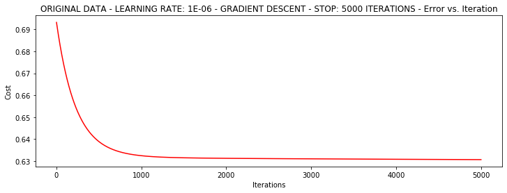
値の損失を止めるためによると
設定された閾値1E-6、ほぼ11万反復が必要
runExpe(orig_data, theta, n, STOP_COST, thresh=0.000001, alpha=0.001)***Original data - learning rate: 0.001 - Gradient descent - Stop: costs change < 1e-06
Theta: [[-5.13364014 0.04771429 0.04072397]] - Iter: 109901 - Last cost: 0.38 - Duration: 32.65s
array([[-5.13364014, 0.04771429, 0.04072397]])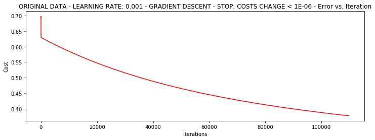
グラデーション停止よると
設定されたしきい値0.05、ほぼ40,000回の反復が必要
runExpe(orig_data, theta, n, STOP_GRAD, thresh=0.05, alpha=0.001)***Original data - learning rate: 0.001 - Gradient descent - Stop: gradient norm < 0.05
Theta: [[-2.37033409 0.02721692 0.01899456]] - Iter: 40045 - Last cost: 0.49 - Duration: 12.20s
array([[-2.37033409, 0.02721692, 0.01899456]])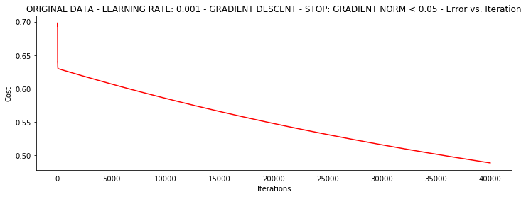
異なる勾配降下法の比較
確率的ディセント
runExpe(orig_data, theta, 1, STOP_ITER, thresh=5000, alpha=0.001)***Original data - learning rate: 0.001 - Stochastic descent - Stop: 5000 iterations
Theta: [[-0.36656341 -0.01406809 -0.01956622]] - Iter: 5000 - Last cost: 1.80 - Duration: 0.45s
array([[-0.36656341, -0.01406809, -0.01956622]])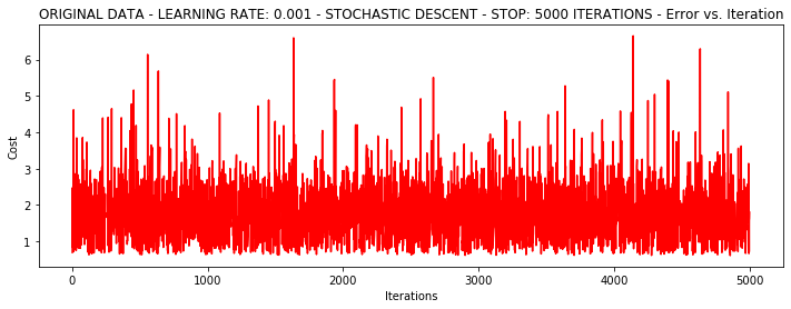
少し爆発。。。非常に不安定、小さな学習率を転送し、再試行してください
runExpe(orig_data, theta, 1, STOP_ITER, thresh=15000, alpha=0.000002)***Original data - learning rate: 2e-06 - Stochastic descent - Stop: 15000 iterations
Theta: [[-0.00202316 0.00991808 0.00087764]] - Iter: 15000 - Last cost: 0.63 - Duration: 1.38s
array([[-0.00202316, 0.00991808, 0.00087764]])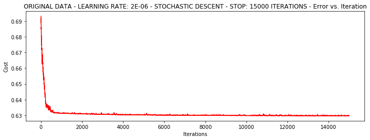
スピード、しかし貧しい安定性は、非常に小さな学習率が必要です
ミニバッチ降下
runExpe(orig_data, theta, 16, STOP_ITER, thresh=15000, alpha=0.001)***Original data - learning rate: 0.001 - Mini-batch (16) descent - Stop: 15000 iterations
Theta: [[-1.03398289 0.04372859 0.02318741]] - Iter: 15000 - Last cost: 1.05 - Duration: 1.83s
array([[-1.03398289, 0.04372859, 0.02318741]])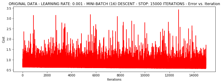
フローティングは、まだ私たちの次のデータを標準化しようとする試みが比較的大きい
分散で割った後、その属性に応じたデータに(列がなかった)マイナス平均値、および。最終結果は、0の近傍で収集されたすべてのデータのそれぞれについて、各属性/列に対して、分散値であります
from sklearn import preprocessing as pp

scaled_data = orig_data.copy()
scaled_data[:, 1:3] = pp.scale(orig_data[:, 1:3])

runExpe(scaled_data, theta, n, STOP_ITER, thresh=5000, alpha=0.001)
***Scaled data - learning rate: 0.001 - Gradient descent - Stop: 5000 iterations
Theta: [[0.3080807 0.86494967 0.77367651]] - Iter: 5000 - Last cost: 0.38 - Duration: 1.56s
array([[0.3080807 , 0.86494967, 0.77367651]])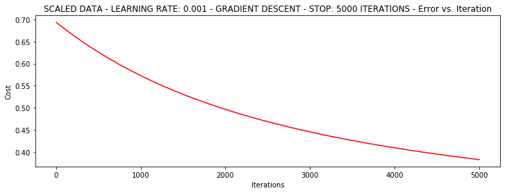
それははるかに優れています!生データは、唯一の到達0.61、0.38に達することができると私たちはここに来ました!
そのため、データの前処理は非常に重要です
runExpe(scaled_data, theta, n, STOP_GRAD, thresh=0.02, alpha=0.001)***Scaled data - learning rate: 0.001 - Gradient descent - Stop: gradient norm < 0.02
Theta: [[1.0707921 2.63030842 2.41079787]] - Iter: 59422 - Last cost: 0.22 - Duration: 19.58s
array([[1.0707921 , 2.63030842, 2.41079787]])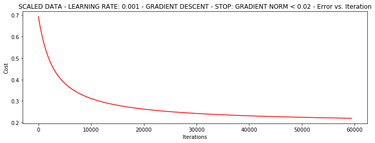
より多くの反復は秋より多くの損失を行います!
theta = runExpe(scaled_data, theta, 1, STOP_GRAD, thresh=0.002/5, alpha=0.001)***Scaled data - learning rate: 0.001 - Stochastic descent - Stop: gradient norm < 0.0004
Theta: [[1.14964649 2.79191694 2.56889202]] - Iter: 72692 - Last cost: 0.22 - Duration: 8.55s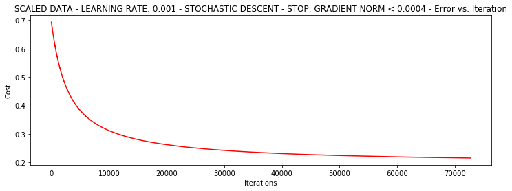
確率的勾配降下より速く、しかし、我々は、彼らがまだバッチがより適切である使用し、より多くの必要な反復回数を必要とします!!!
runExpe(scaled_data, theta, 16, STOP_GRAD, thresh=0.002*2, alpha=0.001)***Scaled data - learning rate: 0.001 - Mini-batch (16) descent - Stop: gradient norm < 0.004
Theta: [[1.15785505 2.80909166 2.5880511 ]] - Iter: 1700 - Last cost: 0.22 - Duration: 0.36s
array([[1.15785505, 2.80909166, 2.5880511 ]])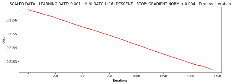
精度
#设定阈值
def predict(X, theta):
    return [1 if x >= 0.5 else 0 for x in model(X, theta)]
scaled_X = scaled_data[:, :3]
y = scaled_data[:, 3]
predictions = predict(scaled_X, theta)
correct = [1 if ((a == 1 and b == 1) or (a == 0 and b == 0)) else 0 for (a, b) in zip(predictions, y)]
accuracy = (sum(map(int, correct)) % len(correct))
print ('accuracy = {0}%'.format(accuracy))accuracy = 89%