目次
1.3.1 テストデータから式行列とアノテーション情報を抽出する
1.4.2 RcisTarget データベース ファイルの初期化
2.2. 遺伝子制御ネットワーク活性 (GRN スコア) の構築と計算
1 インストール
1.1 梱包
SCENICワークフローは主に 3 つの R パッケージのサポートに依存しています:
1. GENIE3: 共発現ネットワークの計算に使用 (GRNBoost2代替としても使用可能)
2. RcisTarget: 転写因子結合モチーフの計算
3. AUCell: 活性化された遺伝子セットの同定単一細胞配列データ (遺伝子ネットワーク)
#安装是个永恒的难题,我在window中BiocManager==1.30.16,R==4.0.6以及本篇的sessionInfo环境下安装是没有问题的
#在Linux中如果你对conda比较熟悉那么也很好安装
if (!requireNamespace("BiocManager", quietly = TRUE))install.packages("BiocManager")
BiocManager::version()
#当你的bioconductor版本大于4.0时
if(!require(SCENIC))BiocManager::install(c("AUCell", "RcisTarget"),ask = F,update = F);BiocManager::install(c("GENIE3"),ask = F,update = F)#这三个包显然是必须安装的

### 可选的包:
#AUCell依赖包
if(!require(SCENIC))BiocManager::install(c("zoo", "mixtools", "rbokeh"),ask = F,update = F)
###t-SNEs计算依赖包:
if(!require(SCENIC))BiocManager::install(c("DT", "NMF", "ComplexHeatmap", "R2HTML", "Rtsne"),ask = F,update = F)

# #这几个包用于并行计算,很遗憾,Windows下并不支持,所以做大量数据计算时最好转战linux:
if(!require(SCENIC))BiocManager::install(c("doMC", "doRNG"),ask = F,update = F)
#可视化输出

# To export/visualize in http://scope.aertslab.org
if (!requireNamespace("devtools", quietly = TRUE))install.packages("devtools")
if(!require(SCopeLoomR))devtools::install_github("aertslab/SCopeLoomR", build_vignettes = TRUE)#SCopeLoomR用于获取测试数据

if (!requireNamespace("arrow", quietly = TRUE)) BiocManager::install('arrow')
#这个包不装上在runSCENIC_2_createRegulons那一步会报错,提示'dbs'不存在
library(SCENIC)#这就安装好了,试试能不能正常加载

if(!require(SCENIC))devtools::install_github("aertslab/SCENIC")
packageVersion("SCENIC")#这里我安装的是1.3.1
library(SCENIC)

#bioconductor版本小于4.0或你的R(3.6)的版本也比较老,你可能得试试下面的方法进行安装
devtools::install_github("aertslab/[email protected]")
devtools::install_github("aertslab/AUCell")
devtools::install_github("aertslab/RcisTarget")
devtools::install_github("aertslab/GENIE3")
1.2 公式マニュアル
vignetteFile <- file.path(system.file('doc', package='SCENIC'), "SCENIC_Running.Rmd")
file.copy(vignetteFile, "SCENIC_myRun.Rmd")
# or:
vignetteFile <- "https://raw.githubusercontent.com/aertslab/SCENIC/master/vignettes/SCENIC_Running.Rmd"
download.file(vignetteFile, "SCENIC_myRun.Rmd")
1.3 テストデータ
1.3.1 テストデータから式行列とアノテーション情報を抽出する
入力データの発現行列は遺伝子要約カウントです。他の高度な分析とは異なり、入力データは生のカウントまたは正規化されたカウントであることが好ましいです。計算されたTPMまたはFPKM/RPKMも許可されますが、これらは人工共変数の導入につながる可能性があります。無関係な問題を避けるために、生のカウントを使用することをお勧めします。ただし、一般に、 生の (ログに記録された) UMI カウント、 正規化された UMI カウント、およびTPMはすべて、信頼できる結果を生成できます。 loom
loomPath <- system.file(package="SCENIC", "examples/mouseBrain_toy.loom")
library(SCopeLoomR)
loom <- open_loom(loomPath)#获取loom文件
exprMat <- get_dgem(loom)#取出表达信息
class(exprMat)# [1] "matrix" "array"exprMat[1:4,1:4]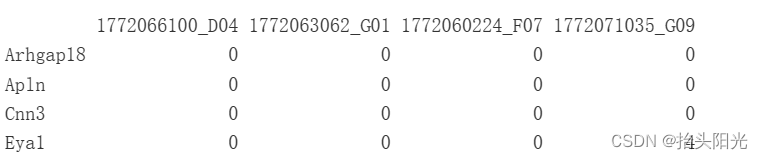
cellInfo <- get_cell_annotation(loom)#获得注释信息
cellInfo[1:4,1:3] 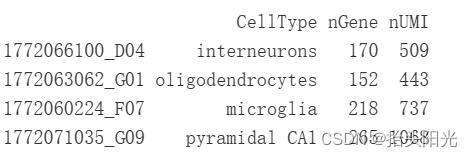
close_loom(loom)上記では、式マトリックスloomとそこから。SCENIC の Python バージョンでは、入力データとして Loom を使用することを推奨しています。ここでは、式マトリックスとアノテーション情報を使用してloomファイルを作成する方法を説明します (〜 loom)
loom <- build_loom("data/mouseBrain.loom", dgem=exprMat)
loom <- SCENIC::add_cell_annotation(loom, cellInfo)close_loom(loom) seuratオブジェクトも似ています
library(Seurat)
singleCellMatrix <- Seurat::Read10X(data.dir="data/filtered_gene_bc_matrices/hg19/")
scRNAsub <- CreateSeuratObject(counts = singleCellMatrix, project = "pbmc3k", min.cells = 3, min.features = 200)
exprMat <- as.matrix(scRNAsub@assays$RNA@counts)
cellInfo <- as.data.frame([email protected])AUCellアノテーション情報を
cellLabels <- paste(file.path(system.file('examples', package='AUCell')), "mouseBrain_cellLabels.tsv", sep="/")
cellLabels <- read.table(cellLabels, row.names=1, header=TRUE, sep="\t")
cellInfo <- as.data.frame(cellLabels)
colnames(cellInfo) <- "CellType"
saveRDS(cellInfo,'int/cellInfo.rds')
1.3.2 入力データの保存
saveRDS(cellInfo, file="int/cellInfo.Rds")
# Color to assign to the variables (same format as for NMF::aheatmap)
colVars <- list(CellType=c("microglia"="forestgreen",
                           "endothelial-mural"="darkorange",
                           "astrocytes_ependymal"="magenta4",
                           "oligodendrocytes"="hotpink",
                           "interneurons"="red3",
                           "pyramidal CA1"="skyblue",
                           "pyramidal SS"="darkblue"))
colVars$CellType <- colVars$CellType[intersect(names(colVars$CellType), cellInfo$CellType)]
saveRDS(colVars, file="int/colVars.Rds")
plot.new(); legend(0,1, fill=colVars$CellType, legend=names(colVars$CellType))#查看保存了哪些细胞类型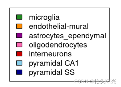
1.4 RcisTargetデータベース
1.4.1 ファイルの取得
cisTarget データベースの マニュアルダウンロード
#地址
#human:
dbFiles <- c("https://resources.aertslab.org/cistarget/databases/homo_sapiens/hg19/refseq_r45/mc9nr/gene_based/hg19-500bp-upstream-7species.mc9nr.feather",
             "https://resources.aertslab.org/cistarget/databases/homo_sapiens/hg19/refseq_r45/mc9nr/gene_based/hg19-tss-centered-10kb-7species.mc9nr.feather")

#mouse:
dbFiles <- c("https://resources.aertslab.org/cistarget/databases/mus_musculus/mm9/refseq_r45/mc9nr/gene_based/mm9-500bp-upstream-7species.mc9nr.feather",
             "https://resources.aertslab.org/cistarget/databases/mus_musculus/mm9/refseq_r45/mc9nr/gene_based/mm9-tss-centered-10kb-7species.mc9nr.feather")


#fly:
dbFiles <- c("https://resources.aertslab.org/cistarget/databases/drosophila_melanogaster/dm6/flybase_r6.02/mc8nr/gene_based/dm6-5kb-upstream-full-tx-11species.mc8nr.feather")

#下载

dir.create("cisTarget_databases"); setwd("cisTarget_databases")
for(featherURL in dbFiles)
{
  download.file(featherURL, destfile=basename(featherURL)) # saved in current dir
}
1.4.2 RcisTargetデータベース ファイルの初期化
この手順は、上でダウンロードしたファイルのインデックスを作成し、いくつかのデフォルト パラメータを設定することと同じです。
### Initialize settings
library(SCENIC)
scenicOptions <- initializeScenic(org="mgi",#mouse填'mgi', human填'hgnc',fly填'dmel')
dbDir="cisTarget_databases/mouse/mouse.mm9/", nCores=8)#这里可以设置并行计算
scenicOptions@inputDatasetInfo$cellInfo <- "int/cellInfo.Rds"
saveRDS(scenicOptions, file="int/scenicOptions.Rds")
2. SCENIC分析プロセス(簡易版)
SCENIC分析プロセスは適切にカプセル化されており、プロセス全体を実行するのに必要なコードは 12 行以内です (ただし、多数のプロセス ファイルと結果ファイルが生成されます)。
以下のサンプル データは非常に高速が、独自のデータを実行する場合は数日かかる場合があります。
loomPath <- system.file(package="SCENIC", "examples/mouseBrain_toy.loom")
library(SCopeLoomR)
loom <- open_loom(loomPath)#获取loom文件
exprMat <- get_dgem(loom)#取出表达信息
cellInfo <- get_cell_annotation(loom)#获得注释信息2.1. 共発現ネットワークの計算
genesKept <- geneFiltering(exprMat, scenicOptions)
exprMat_filtered <- exprMat[genesKept, ]
runCorrelation(exprMat_filtered, scenicOptions)
exprMat_filtered_log <- log2(exprMat_filtered+1)
# 基因共表达网络计算
mymethod <- 'runGenie3' # 'grnboost2'
library(reticulate)
if(mymethod=='runGenie3'){
runGenie3(exprMat_filtered_log, scenicOptions)
}else{
arb.algo = import('arboreto.algo')
tf_names = getDbTfs(scenicOptions)
tf_names = Seurat::CaseMatch(
search = tf_names,
match = rownames(exprMat_filtered))
adj = arb.algo$grnboost2(
as.data.frame(t(as.matrix(exprMat_filtered))),
tf_names=tf_names, seed=2023L
)
colnames(adj) = c('TF','Target','weight')
saveRDS(adj,file=getIntName(scenicOptions,
'genie3ll'))
}
2.2. 遺伝子制御ネットワーク活性 (GRN スコア) の構築と計算
exprMat_log <- log2(exprMat+1)
scenicOptions@settings$dbs <- scenicOptions@settings$dbs["10kb"] # Toy run settings
scenicOptions <- runSCENIC_1_coexNetwork2modules(scenicOptions)
scenicOptions <- runSCENIC_2_createRegulons(scenicOptions, coexMethod=c("top5perTarget")) # Toy run settings
scenicOptions <- runSCENIC_3_scoreCells(scenicOptions, exprMat_log)
# 通过交互的shiny app选择判定二元矩阵的阈值,这里Rmarkdown不便展示,大家可以自行尝试一下
# aucellApp <- plotTsne_AUCellApp(scenicOptions, exprMat_log)
# savedSelections <- shiny::runApp(aucellApp)
# newThresholds <- savedSelections$thresholds
# scenicOptions@fileNames$int["aucell_thresholds",1] <- "int/newThresholds.Rds"
# saveRDS(newThresholds, file=getIntName(scenicOptions, "aucell_thresholds"))

scenicOptions <- runSCENIC_4_aucell_binarize(scenicOptions)#将AUCell矩阵二元化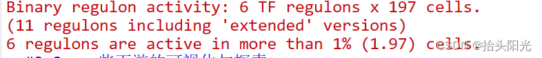
2.3. 下流の視覚化と調査
tsneAUC(scenicOptions, aucType="AUC") #利用AUCell score运行tsne![]()
# Export:
# saveRDS(cellInfo, file=getDatasetInfo(scenicOptions, "cellInfo")) # Temporary, to add to loom
if(!file.exists('output/scenic.loom')){export2loom(scenicOptions, exprMat)}

saveRDS(scenicOptions, file="int/scenicOptions.Rds")#保存结果

### Exploring output
# output下存放的scenic.loom文件可以用这个网站做交互式的可视化: http://scope.aertslab.org

# motif富集的相关信息在:
#output/Step2_MotifEnrichment_preview.html in
motifEnrichment_selfMotifs_wGenes <- loadInt(scenicOptions, "motifEnrichment_selfMotifs_wGenes")
tableSubset <- motifEnrichment_selfMotifs_wGenes[highlightedTFs=="Sox8"]#这样查看Sox8的信息
viewMotifs(tableSubset) 
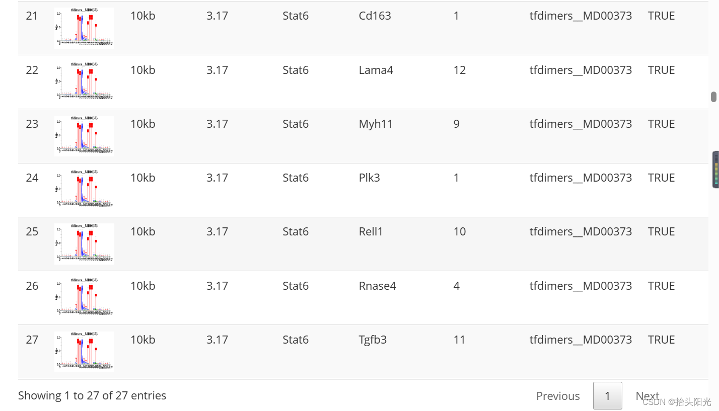
#查看motif和对应基因:
#output/Step2_regulonTargetsInfo.tsv
regulonTargetsInfo <- loadInt(scenicOptions, "regulonTargetsInfo")
tableSubset <- regulonTargetsInfo[TF=="Stat6" & highConfAnnot==TRUE]
viewMotifs(tableSubset) 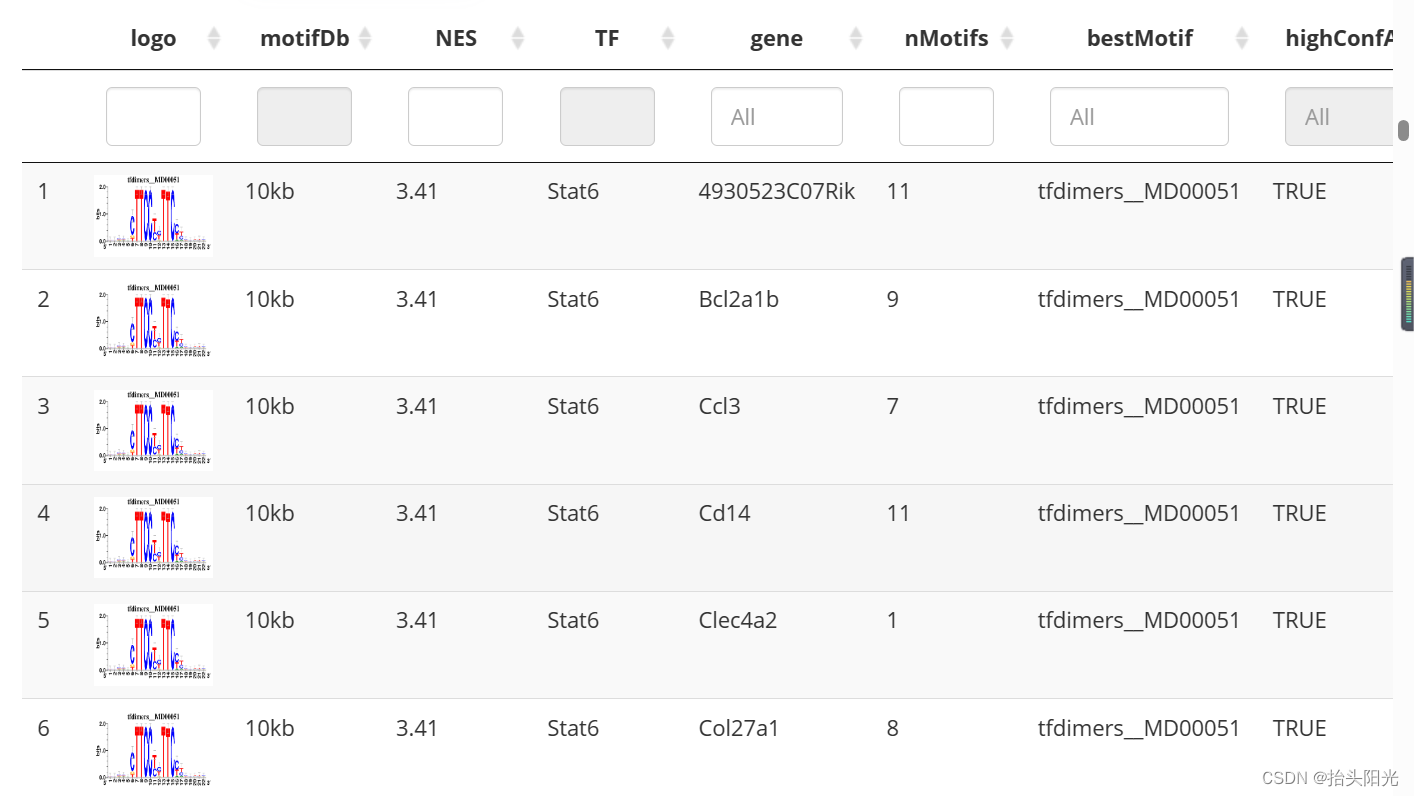
#计算并展示每种细胞类型特异性的(celltype Cell-type specific regulators (RSS)),类似于拿RGN的活性来计算调控
regulonAUC <- loadInt(scenicOptions, "aucell_regulonAUC")
rss <- calcRSS(AUC=getAUC(regulonAUC), cellAnnotation=cellInfo[colnames(regulonAUC), "CellType"], )
rssPlot <- plotRSS(rss)
plotly::ggplotly(rssPlot$plot)
2.4 出力ファイル
上で視覚的に表示した結果に加えて、SCENIC実行時に多数のファイルがローカルに自動的に出力されます。