1. t-SNEの定義

t-SNE は、t-distributed Stochastic Neighbor Embedding の略で、
t-distributed Stochastic Neighbor Embedding を表します。

t-SNE は高次元データを取得し、データポイント間の関係を元の配置にできる限り近づけながら、それを低次元空間に縮小します。

これは、Laurens van der Maaten と Geoffery Hinton によって 2008 年に開発された教師なし機械学習アルゴリズムです。

これが t-SNE の仕組みです。手順は簡単です。

1.1. 高次元空間における類似性の計測

まず、t-SNE は元の高次元空間内のデータポイント間の類似性を測定します。
点間のペアごとの距離を計算し、ガウス分布を使用してそれらを確率に変換します。
確率は、2 つの点が互いに隣接する可能性を表します。

1.2 低次元空間における類似性の表現

次に、t-SNE は低次元空間 (2D または 3D) を作成し、各データポイントのランダムな座標を初期化します。
次に、低次元空間内のこれらの点間のペアごとの距離を計算し、t 分布を使用してそれらを確率に変換します。

1.3 最適化

目標は、低次元空間の確率を高次元空間の確率と同様にすることです。

これは、2 つの確率分布間の差を測定するカルバックライブラー (KL) 発散と呼ばれるコスト関数を最小化する勾配降下法によって行われます。

1.4 t-SNE は主成分分析 (PCA) とどう違うのですか?

t-SNE は、PCA (線形次元削減アルゴリズム) とは異なり、非線形次元削減アルゴリズムです。

主成分分析 (PCA) ではデータに線形関係があると想定されていますが、t-SNE はそうではありません。

したがって、t-SNE は、現実世界の非線形データの次元削減にさらに役立ちます。

2. 各種業務例

2.1 Iris データセット Iris の t-SNE

アヤメデータセットには、Iris variegata、Iris variegata、Iris virginia の 3 つの異なる種のアヤメの 150 サンプルが含まれています。

各サンプルには、がく片の長さ、がく片の幅、花弁の長さ、花びらの幅の 4 つの特徴があります。

このデータセットに 4 次元表現を 2 次元表現に変換する t-SNE を適用した後に得られた結果を視覚化してみましょう。

import numpy as np
import matplotlib.pyplot as plt
from sklearn.datasets import load_iris
from sklearn.manifold import TSNE

# Load the Iris dataset
iris = load_iris()
X, y = iris.data, iris.target

# Perform t-SNE
tsne = TSNE(n_components=2, perplexity=30, random_state=42)
X_tsne = tsne.fit_transform(X)

# Visualize the results
plt.figure(figsize=(8, 6))
scatter = plt.scatter(X_tsne[:, 0], X_tsne[:, 1], c=y, cmap="viridis", alpha=0.8)

cbar = plt.colorbar(scatter, ticks=range(3))
cbar.ax.set_yticklabels(['Iris setosa', 'Iris versicolor', 'Iris virginica']) 

plt.title("Iris Dataset t-SNE Visualization")
plt.xlabel("t-SNE 1st Component")
plt.ylabel("t-SNE 2nd Component")
plt.show()

Perplexity? 什么是困惑度？

perplexity は、高次元空間で確率分布を構築するときに各データポイントで考慮される近傍の数を決定するために t-SNE で使用されるハイパーパラメーターです。

t-SNE を虹彩データセットに適用すると、結果として得られるプロットには、3 つの虹彩種に対応する 3 つの異なるクラスターが表示されます。
ここに画像の説明を挿入
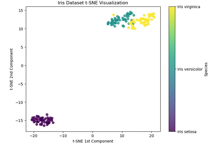
Iris versicolor と Iris virginica の組成が重複していることに注意してください。これは、これらの種間の類似性がさらに高いことを示唆しています。

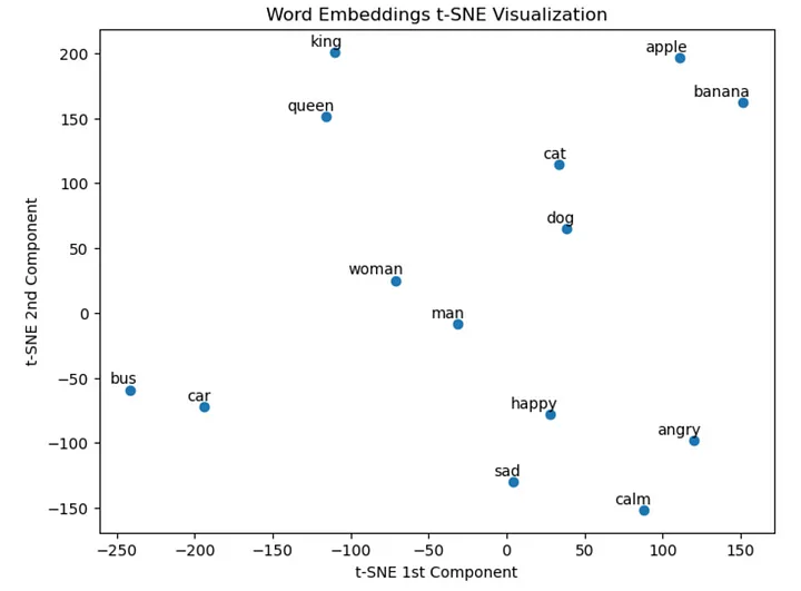
2.2 GloVe 埋め込み上の t-SNE

GloVe (単語表現のためのグローバルベクトル)、

GloVe (Global Vectors of Word Representations) は、単語のベクトル表現 (埋め込みとも呼ばれます) を取得するための教師なし学習アルゴリズムです。

これらの埋め込みは多次元であることに注意してください。t-SNE は 2 次元で使用されます。

import numpy as np
import matplotlib.pyplot as plt
from sklearn.manifold import TSNE
from gensim.downloader import load

# Load the pre-trained GloVe word embeddings
glove_vectors = load("glove-wiki-gigaword-50")

# Select a subset of words to visualize
words_to_visualize = ["king", "queen", "man", "woman", "dog", "cat", "car", "bus", "apple", "banana", "happy", "sad", "angry", "calm"]

# Get the corresponding word vectors
word_vectors = np.array([glove_vectors[word] for word in words_to_visualize])

# Perform t-SNE
tsne = TSNE(n_components=2, perplexity=5, random_state=42)
word_vectors_tsne = tsne.fit_transform(word_vectors)

# Visualize the results
plt.figure(figsize=(8, 6))
scatter = plt.scatter(word_vectors_tsne[:, 0], word_vectors_tsne[:, 1])

# Add labels to the points
for i, word in enumerate(words_to_visualize):
    plt.annotate(word, xy=(word_vectors_tsne[i, 0], word_vectors_tsne[i, 1]), xytext=(5, 2), textcoords="offset points", ha="right", va="bottom")

plt.title("Word Embeddings t-SNE Visualization")
plt.xlabel("t-SNE 1st Component")
plt.ylabel("t-SNE 2nd Component")

plt.show()

ここに画像の説明を挿入

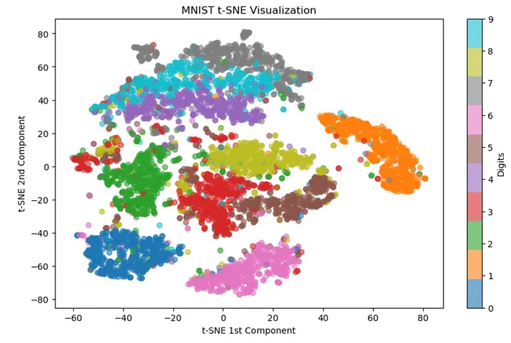
2.3 MNIST データセット MNIST 上の t-SNE

MNIST データセットは、0 から 9 までの 70,000 個の手書きの数字で構成され、それぞれが 28x28 ピクセルのグレースケール画像として表されます。

各画像は 784 次元のベクトル ( 28 * 28 = 784 ) として表されます。

これらの画像を 2D 空間で視覚化してみましょう。

import numpy as np
import matplotlib.pyplot as plt
from sklearn.datasets import fetch_openml
from sklearn.decomposition import PCA
from sklearn.manifold import TSNE
from sklearn.model_selection import train_test_split
from sklearn.preprocessing import StandardScaler

# Load the MNIST dataset
mnist = fetch_openml("mnist_784")
X, y = mnist.data, mnist.target

最初に StandardScaler を使用してデータをスケーリングし、次に計算を高速化するために 5000 枚の画像のサブセットを選択することに注意してください。

# Preprocess the data
scaler = StandardScaler()
X_scaled = scaler.fit_transform(X)

# Select a subset of the dataset for faster computation
X_subset, _, y_subset, _ = train_test_split(X_scaled, y, train_size=5000, random_state=42, stratify=y)

t-SNE の sklearn ドキュメントには、特徴の数が非常に多い場合、別の次元削減方法 (PCA など) を使用して次元数を適切な数 (50 など) に削減することを強く推奨することが記載されています。高い (この場合は 784)。

したがって、t-SNE を適用する前に、PCA を使用して MNIST データセットの次元を 784 次元から 50 次元に削減します。

# Perform PCA for faster t-SNE computation
pca = PCA(n_components=50)
X_pca = pca.fit_transform(X_subset)

次に、t-SNE を実行して結果を視覚化してみましょう。

# Perform t-SNE
tsne = TSNE(n_components=2, perplexity=30, random_state=42)
X_tsne = tsne.fit_transform(X_pca)

# Visualize the results
plt.figure(figsize=(12, 8))
scatter = plt.scatter(X_tsne[:, 0], X_tsne[:, 1], c=y_subset.astype(int), cmap="tab10", alpha=0.6)
plt.colorbar(scatter, ticks=range(10), label="Digits")
plt.title("MNIST t-SNE Visualization")
plt.xlabel("t-SNE 1st Component")
plt.ylabel("t-SNE 2nd Component")
plt.show()