著者:タルン・グプタ
翻訳グループdeephub:孟Xiangjie
この記事では、勾配降下法を使用して(バッチ)線形回帰を実装する方法を学ぶためのpython3データ処理ライブラリで書かれたプログラムとしてnumpyのを使用するようになります。
私は徐々に動作原理とコードのコードの各部分の原理を説明します。
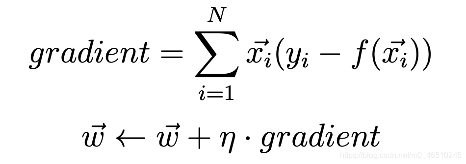
私たちは、勾配を計算し、この計算式を使用します。
ここで、x(i)は、Nはデータセットのサイズである点のベクトルです。N(ETA)は、当社の学習率です。Y(i)が目標出力ベクトルです。F(X)は、シグマは和関数である線形回帰関数のベクトルf(X)=合計(* X W)と定義されます。さらに、我々は最初の違いW0 = 0となるようにX0 = 1を検討します。すべての重みは0に初期化されています。
この方法では、我々は、二乗誤差損失関数の合計を使用しました。
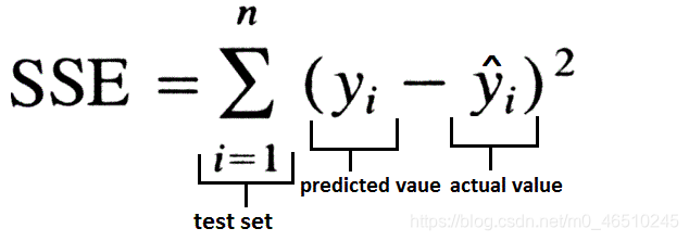
SSEはゼロに初期化されていることを除いて、我々は、SSEの各反復の変化を記録し、プログラムの実行に先立って閾値と比較されます。SSEが閾値を下回る場合、プログラムは終了します。
このプログラムでは、コマンドラインから3つの入力を提供します。彼らは以下のとおりです。
しきい値 -しきい値は、アルゴリズムが終了する前に、損失がこのしきい値未満でなければなりません。
データ -データセットの位置。
learningRate -学習率勾配降下方法。
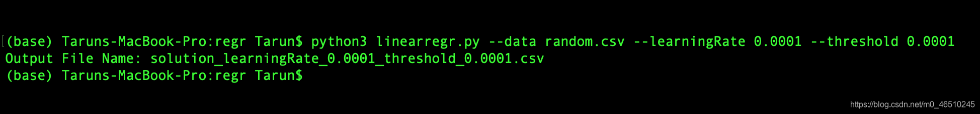
そのため、プログラムの開始は、次のようになります。
python3linearregr.py — datarandom.csv — learningRate 0.0001 — threshold 0.0001
次のように我々は最後のものを識別コードに入る前に、プログラムの出力は次のようになります。
iteration_number,weight0,weight1,weight2,...,weightN,sum_of_squared_errors
プログラムは6つの部分、私たちが見る一つ一つを含んでいます。
インポートモジュール
import argparse # to read inputs from command lineimport csv # to read the input data set fileimport numpy as np # to work with the data set
初期化部
# initialise argument parser and read argumentsfrom command line with the respective flags and then call the main() functionif __name__ == '__main__':
    parser = argparse.ArgumentParser()
    parser.add_argument("-d", "--data", help="Data File")
    parser.add_argument("-l", "--learningRate", help="Learning Rate")
    parser.add_argument("-t", "--threshold", help="Threshold")
    main()
主な機能の一部
defmain():
    args = parser.parse_args()
    file, learningRate, threshold = args.data, float(
        args.learningRate), float(args.threshold) # save respective command line inputs into variables# read csv file and the last column is the target output and is separated from the input (X) as Ywith open(file) as csvFile:
        reader = csv.reader(csvFile, delimiter=',')
        X = []
        Y = []
        for row in reader:
            X.append([1.0] + row[:-1])
            Y.append([row[-1]])

    # Convert data points into float and initialise weight vector with 0s.
    n = len(X)
    X = np.array(X).astype(float)
    Y = np.array(Y).astype(float)
    W = np.zeros(X.shape[1]).astype(float)
    # this matrix is transposed to match the necessary matrix dimensions for calculating dot product
    W = W.reshape(X.shape[1], 1).round(4)

    # Calculate the predicted output value
    f_x = calculatePredicatedValue(X, W)

    # Calculate the initial SSE
    sse_old = calculateSSE(Y, f_x)

    outputFile = 'solution_' + \
                 'learningRate_' + str(learningRate) + '_threshold_' \
                 + str(threshold) + '.csv''''
        Output file is opened in writing mode and the data is written in the format mentioned in the post. After the
        first values are written, the gradient and updated weights are calculated using the calculateGradient function.
        An iteration variable is maintained to keep track on the number of times the batch linear regression is executed
        before it falls below the threshold value. In the infinite while loop, the predicted output value is calculated
        again and new SSE value is calculated. If the absolute difference between the older(SSE from previous iteration)
        and newer(SSE from current iteration) SSE is greater than the threshold value, then above process is repeated.
        The iteration is incremented by 1 and the current SSE is stored into previous SSE. If the absolute difference
        between the older(SSE from previous iteration) and newer(SSE from current iteration) SSE falls below the
        threshold value, the loop breaks and the last output values are written to the file.
    '''with open(outputFile, 'w', newline='') as csvFile:
        writer = csv.writer(csvFile, delimiter=',', quoting=csv.QUOTE_NONE, escapechar='')
        writer.writerow([*[0], *["{0:.4f}".format(val) for val in W.T[0]], *["{0:.4f}".format(sse_old)]])

        gradient, W = calculateGradient(W, X, Y, f_x, learningRate)

        iteration = 1whileTrue:
            f_x = calculatePredicatedValue(X, W)
            sse_new = calculateSSE(Y, f_x)

            if abs(sse_new - sse_old) > threshold:
                writer.writerow([*[iteration], *["{0:.4f}".format(val) for val in W.T[0]], *["{0:.4f}".format(sse_new)]])
                gradient, W = calculateGradient(W, X, Y, f_x, learningRate)
                iteration += 1
                sse_old = sse_new
            else:
                break
        writer.writerow([*[iteration], *["{0:.4f}".format(val) for val in W.T[0]], *["{0:.4f}".format(sse_new)]])
    print("Output File Name: " + outputFile
次のようにプロセス主な機能は次のとおりです。
- 変数への入力に対応するコマンドライン
- CSVファイルを読み込む、最後のものが目標出力、および(Xとして格納されている)の入力と別Yとして記憶されます
- データ点は0の重みの浮動小数点初期化ベクトルに変換します
- 出力の予測値を計算するために使用calculatePredicatedValue機能
- SSE機能は初期calculateSSEを計算するために使用されます
- 出力ファイルを書き込みモードでオープンされ、データは記事で述べた形式で記述されています。最初の値を書き込み、calculateGradient更新重みを計算勾配機能を使用した後。反復の可変数が閾値未満の損失関数値の前に一括して行う線形回帰を決定するために行わ。無限ループで、再度予測出力値を算出し、SSEの新しい値を計算します。古い(SSEから前の反復)及び(現在の反復からSSE)との間の新しい絶対差が閾値より大きい場合、処理を繰り返します。反復1の数を増やし、SSEは現在、以前SSEに記憶されています。古い(SSEの前の反復)及び(SSEの現在の反復)との間の新しい絶対差がしきい値未満である場合、サイクルが中断され、ファイルに書き込まれ、最終的な出力値です。
calculatePredicatedValue機能
ここで、生成物は、予測出力を実行することによって計算され、入力行列X Wは重み行列点です。
# dot product of X(input) and W(weights) as numpy matrices and returning the result which is the predicted outputdefcalculatePredicatedValue(X, W):
    f_x = np.dot(X, W)
    return f_x
calculateGradient機能
勾配は、最初の記事に記載された式を用いて計算し、重みを更新します。
defcalculateGradient(W, X, Y, f_x, learningRate):
    gradient = (Y - f_x) * X
    gradient = np.sum(gradient, axis=0)
    temp = np.array(learningRate * gradient).reshape(W.shape)
    W = W + temp
    return gradient, W
calculateSSE機能
SSEは、上記の式を用いて計算されます。
defcalculateSSE(Y, f_x):
    sse = np.sum(np.square(f_x - Y))
    return sse
さて、完全なコードを読みます。プログラムの実施の結果で見てみましょう。
これは出力のようなものです:
00.00000.00000.00007475.31491-0.0940-0.5376-0.25922111.51052-0.1789-0.7849-0.3766880.69803-0.2555-0.8988-0.4296538.86384-0.3245-0.9514-0.4533399.80925-0.3867-0.9758-0.4637316.16826-0.4426-0.9872- 0.4682254.51267-0.4930-0.9926-0.4699205.84798-0.5383-0.9952-0.4704166.69329-0.5791-0.9966-0.4704135.029310-0.6158-0.9973-0.4702109.389211-0.6489-0.9978-0.470088.619712-0.6786-0.9981-0.469771。 794113-0.7054-0.9983-0.469458.163114-0.7295-0.9985-0.469147.120115-0.7512-0.9987-0.468938.173816-0.7708-0.9988-0.468730.926117-0.7883-0.9989-0.468525.054418-0.8042-0.9990-0.468320.297519- 0.8184-0.9991-0.468116.443820-0.8312-0.9992-0.468013.321821-0.8427-0.9993-0.467810.792522-0.8531-0.9994-0.46778.743423-0.8625-0.9994-0.46767.083324-0.8709-0.9995-0.46755.738525-0.8785- 0.9995-0.46744.649026-0.8853-0.9996-0.46743.766327-0.8914-0.9996-0.46733.051228-0.8969-0.9997-0.46722。471929-0.9019-0.9997-0.46722.002630-0.9064-0.9997-0.46711.622431-0.9104-0.9998-0.46711.314432-0.9140-0.9998-0.46701.064833-0.9173-0.9998-0.46700.862634-0.9202-0.9998-0.46700.698935- 0.9229-0.9998-0.46690.566236-0.9252-0.9999-0.46690.458737-0.9274-0.9999-0.46690.371638-0.9293-0.9999-0.46690.301039-0.9310-0.9999-0.46680.243940-0.9326-0.9999-0.46680.197641-0.9340- 0.9999-0.46680.160142-0.9353-0.9999-0.46680.129743-0.9364-0.9999-0.46680.105144-0.9374-0.9999-0.46680.085145-0.9384-0.9999-0.46680.069046-0.9392-0.9999-0.46680.055947-0.9399-1.0000- 0.46670.045348-0.9406-1.0000-0.46670.036749-0.9412-1.0000-0.46670.029750-0.9418-1.0000-0.46670.024151-0.9423-1.0000-0.46670.019552-0.9427-1.0000-0.46670.015853-0.9431-1.0000-0.46670。 012854-0.9434-1.0000-0.46670.010455-0.9438-1.0000-0.46670.008456-0.9441-1.0000-0.46670.006857-0.9443-1.0000-0.46670.005558-0.9446-1。0000-0.46670.004559-0.9448-1.0000-0.46670.003660-0.9450-1.0000-0.46670.002961-0.9451-1.0000-0.46670.002462-0.9453-1.0000-0.46670.001963-0.9454-1.0000-0.46670.001664-0.9455-1.0000- 0.46670.001365-0.9457-1.0000-0.46670.001066-0.9458-1.0000-0.46670.000867-0.9458-1.0000-0.46670.000768-0.9459-1.0000-0.46670.000569-0.9460-1.0000-0.46670.000470-0.9461-1.0000-0.46670。 0004
最終案
import argparse
import csv
import numpy as np


defmain():
    args = parser.parse_args()
    file, learningRate, threshold = args.data, float(
        args.learningRate), float(args.threshold) # save respective command line inputs into variables# read csv file and the last column is the target output and is separated from the input (X) as Ywith open(file) as csvFile:
        reader = csv.reader(csvFile, delimiter=',')
        X = []
        Y = []
        for row in reader:
            X.append([1.0] + row[:-1])
            Y.append([row[-1]])

    # Convert data points into float and initialise weight vector with 0s.
    n = len(X)
    X = np.array(X).astype(float)
    Y = np.array(Y).astype(float)
    W = np.zeros(X.shape[1]).astype(float)
    # this matrix is transposed to match the necessary matrix dimensions for calculating dot product
    W = W.reshape(X.shape[1], 1).round(4)

    # Calculate the predicted output value
    f_x = calculatePredicatedValue(X, W)

    # Calculate the initial SSE
    sse_old = calculateSSE(Y, f_x)

    outputFile = 'solution_' + \
                 'learningRate_' + str(learningRate) + '_threshold_' \
                 + str(threshold) + '.csv''''
        Output file is opened in writing mode and the data is written in the format mentioned in the post. After the
        first values are written, the gradient and updated weights are calculated using the calculateGradient function.
        An iteration variable is maintained to keep track on the number of times the batch linear regression is executed
        before it falls below the threshold value. In the infinite while loop, the predicted output value is calculated
        again and new SSE value is calculated. If the absolute difference between the older(SSE from previous iteration)
        and newer(SSE from current iteration) SSE is greater than the threshold value, then above process is repeated.
        The iteration is incremented by 1 and the current SSE is stored into previous SSE. If the absolute difference
        between the older(SSE from previous iteration) and newer(SSE from current iteration) SSE falls below the
        threshold value, the loop breaks and the last output values are written to the file.
    '''with open(outputFile, 'w', newline='') as csvFile:
        writer = csv.writer(csvFile, delimiter=',', quoting=csv.QUOTE_NONE, escapechar='')
        writer.writerow([*[0], *["{0:.4f}".format(val) for val in W.T[0]], *["{0:.4f}".format(sse_old)]])

        gradient, W = calculateGradient(W, X, Y, f_x, learningRate)

        iteration = 1whileTrue:
            f_x = calculatePredicatedValue(X, W)
            sse_new = calculateSSE(Y, f_x)

            if abs(sse_new - sse_old) > threshold:
                writer.writerow([*[iteration], *["{0:.4f}".format(val) for val in W.T[0]], *["{0:.4f}".format(sse_new)]])
                gradient, W = calculateGradient(W, X, Y, f_x, learningRate)
                iteration += 1
                sse_old = sse_new
            else:
                break
        writer.writerow([*[iteration], *["{0:.4f}".format(val) for val in W.T[0]], *["{0:.4f}".format(sse_new)]])
    print("Output File Name: " + outputFile


defcalculateGradient(W, X, Y, f_x, learningRate):
    gradient = (Y - f_x) * X
    gradient = np.sum(gradient, axis=0)
    # gradient = np.array([float("{0:.4f}".format(val)) for val in gradient])
    temp = np.array(learningRate * gradient).reshape(W.shape)
    W = W + temp
    return gradient, W


defcalculateSSE(Y, f_x):
    sse = np.sum(np.square(f_x - Y))

    return sse


defcalculatePredicatedValue(X, W):
    f_x = np.dot(X, W)
    return f_x


if __name__ == '__main__':
    parser = argparse.ArgumentParser()
    parser.add_argument("-d", "--data", help="Data File")
    parser.add_argument("-l", "--learningRate", help="Learning Rate")
    parser.add_argument("-t", "--threshold", help="Threshold")
    main()
この記事では、バッチ線形回帰の勾配降下法を用いた数学的概念を説明しています。ここでは、(二乗誤差の合計として、この場合)損失関数を考えます。私たちは、SSEを最小限にする方法を参照していない、これは(学習率を調整するために)起こるべきではありません、我々は、しきい値の助けを借りて、線形回帰の方法収束を見ました。
プログラムは、numpyのプロセスデータを使用して完全にPythonのnumpyのの基礎を使用することなく使用することができるが、それは、ネストされたループが必要になり、時間がOの複雑さを増加させる(N * N)であろう。いずれの場合においても、より高いメモリ効率numpyのアレイとマトリックスは提供しました。あなたはパンダモジュールを使用することを好む場合も、私たちは、あなたがそれを使用することをお勧めします、と同じ手順を達成するためにそれを使用してみてください。
私はあなたがこの記事を楽しんだことを望みます。読んでくれてありがとう。