[Construir la red neuronal PyTorch para la predicción de temperatura]

import numpy as np
import pandas as pd 
import matplotlib.pyplot as plt
import torch
import torch.optim as optim
import warnings
warnings.filterwarnings("ignore")
%matplotlib inline

features = pd.read_csv('temps.csv')

#看看数据长什么样子
features.head()

	año	mes	día	semana	temp_2	temp_1	promedio	actual	amigo
0	2016	1	1	Vie	45	45	45.6	45	29
1	2016	1	2	Se sentó	44	45	45.7	44	61
2	2016	1	3	Sol	45	44	45,8	41	56
3	2016	1	4	Lun	44	41	45,9	40	53
4	2016	1	5	martes	41	40	46,0	44	41

en la hoja de datos

• El tiempo específico representado por año, mes, día y semana respectivamente
• temp_2: el valor de temperatura más alto de anteayer
• temp_1: valor de temperatura más alto de ayer
• promedio: en la historia, el valor promedio de la temperatura máxima de este día cada año
• actual: Este es nuestro valor de etiqueta, la temperatura máxima real del día
• amigo: esta columna puede ser por diversión, el posible valor adivinado por su amigo, simplemente ignorémoslo

print('数据维度:', features.shape)

数据维度: (348, 9)

# 处理时间数据
import datetime

# 分别得到年，月，日
years = features['year']
months = features['month']
days = features['day']

# datetime格式
dates = [str(int(year)) + '-' + str(int(month)) + '-' + str(int(day)) for year, month, day in zip(years, months, days)]
dates = [datetime.datetime.strptime(date, '%Y-%m-%d') for date in dates]

dates[:5]

[datetime.datetime(2016, 1, 1, 0, 0),
 datetime.datetime(2016, 1, 2, 0, 0),
 datetime.datetime(2016, 1, 3, 0, 0),
 datetime.datetime(2016, 1, 4, 0, 0),
 datetime.datetime(2016, 1, 5, 0, 0)]

# 准备画图
# 指定默认风格
plt.style.use('fivethirtyeight')

# 设置布局
fig, ((ax1, ax2), (ax3, ax4)) = plt.subplots(nrows=2, ncols=2, figsize = (10,10))
fig.autofmt_xdate(rotation = 45) #x标签倾斜45度

# 标签值
ax1.plot(dates, features['actual'])
ax1.set_xlabel(''); ax1.set_ylabel('Temperature'); ax1.set_title('Max Temp')

# 昨天
ax2.plot(dates, features['temp_1'])
ax2.set_xlabel(''); ax2.set_ylabel('Temperature'); ax2.set_title('Previous Max Temp')

# 前天
ax3.plot(dates, features['temp_2'])
ax3.set_xlabel('Date'); ax3.set_ylabel('Temperature'); ax3.set_title('Two Days Prior Max Temp')

# 我的逗逼朋友
ax4.plot(dates, features['friend'])
ax4.set_xlabel('Date'); ax4.set_ylabel('Temperature'); ax4.set_title('Friend Estimate')

plt.tight_layout(pad=2)

# 独热编码
features = pd.get_dummies(features)
features.head(5)

	año	mes	día	temp_2	temp_1	promedio	actual	amigo	semana_vie	lunes_semana	semana_sáb	semana_dom	semana_jueves	semana_martes	semana_miércoles
0	2016	1	1	45	45	45.6	45	29	1	0	0	0	0	0	0
1	2016	1	2	44	45	45.7	44	61	0	0	1	0	0	0	0
2	2016	1	3	45	44	45,8	41	56	0	0	0	1	0	0	0
3	2016	1	4	44	41	45,9	40	53	0	1	0	0	0	0	0
4	2016	1	5	41	40	46,0	44	41	0	0	0	0	0	1	0

# 标签
labels = np.array(features['actual'])

# 在特征中去掉标签
features= features.drop('actual', axis = 1)

# 名字单独保存一下，以备后患
feature_list = list(features.columns)

# 转换成合适的格式
features = np.array(features)

features.shape

(348, 14)

from sklearn import preprocessing
input_features = preprocessing.StandardScaler().fit_transform(features)

input_features[0]

array([ 0.        , -1.5678393 , -1.65682171, -1.48452388, -1.49443549,
       -1.3470703 , -1.98891668,  2.44131112, -0.40482045, -0.40961596,
       -0.40482045, -0.40482045, -0.41913682, -0.40482045])

Construir un modelo de red

[La transferencia de la imagen del enlace externo falló, el sitio de origen puede tener un mecanismo anti-leeching, se recomienda guardar la imagen y cargarla directamente (img-I9ez3tyG-1691437809583) (archivo adjunto: imagen.png)]

#将数据转化为tensor的形式
x = torch.tensor(input_features, dtype = float)

y = torch.tensor(labels, dtype = float)

# 权重参数初始化
weights = torch.randn((14, 128), dtype = float, requires_grad = True) 
biases = torch.randn(128, dtype = float, requires_grad = True) 
weights2 = torch.randn((128, 1), dtype = float, requires_grad = True) 
biases2 = torch.randn(1, dtype = float, requires_grad = True) 

learning_rate = 0.001 
losses = []

for i in range(1000):
    # 计算隐层
    hidden = x.mm(weights) + biases
    # 加入激活函数
    hidden = torch.relu(hidden)
    # 预测结果
    predictions = hidden.mm(weights2) + biases2
    # 通计算损失
    loss = torch.mean((predictions - y) ** 2) 
    losses.append(loss.data.numpy())
    
    # 打印损失值
    if i % 100 == 0:
        print('loss:', loss)
    #返向传播计算
    loss.backward()
    
    #更新参数
    weights.data.add_(- learning_rate * weights.grad.data)  
    biases.data.add_(- learning_rate * biases.grad.data)
    weights2.data.add_(- learning_rate * weights2.grad.data)
    biases2.data.add_(- learning_rate * biases2.grad.data)
    
    # 每次迭代都得记得清空
    weights.grad.data.zero_()
    biases.grad.data.zero_()
    weights2.grad.data.zero_()
    biases2.grad.data.zero_()

loss: tensor(4238.8822, dtype=torch.float64, grad_fn=<MeanBackward0>)
loss: tensor(155.8961, dtype=torch.float64, grad_fn=<MeanBackward0>)
loss: tensor(146.9377, dtype=torch.float64, grad_fn=<MeanBackward0>)
loss: tensor(144.1912, dtype=torch.float64, grad_fn=<MeanBackward0>)
loss: tensor(142.8590, dtype=torch.float64, grad_fn=<MeanBackward0>)
loss: tensor(142.0588, dtype=torch.float64, grad_fn=<MeanBackward0>)
loss: tensor(141.5304, dtype=torch.float64, grad_fn=<MeanBackward0>)
loss: tensor(141.1626, dtype=torch.float64, grad_fn=<MeanBackward0>)
loss: tensor(140.8778, dtype=torch.float64, grad_fn=<MeanBackward0>)
loss: tensor(140.6519, dtype=torch.float64, grad_fn=<MeanBackward0>)

predictions.shape

torch.Size([348, 1])

Modelos de red más fáciles de construir

input_size = input_features.shape[1]
hidden_size = 128
output_size = 1
batch_size = 16
my_nn = torch.nn.Sequential(
    torch.nn.Linear(input_size, hidden_size),
    torch.nn.Sigmoid(),
    torch.nn.Linear(hidden_size, output_size),
)
cost = torch.nn.MSELoss(reduction='mean')
optimizer = torch.optim.Adam(my_nn.parameters(), lr = 0.001)

# 训练网络
losses = []
for i in range(1000):
    batch_loss = []
    # MINI-Batch方法来进行训练
    for start in range(0, len(input_features), batch_size):
        end = start + batch_size if start + batch_size < len(input_features) else len(input_features)
        xx = torch.tensor(input_features[start:end], dtype = torch.float, requires_grad = True)
        yy = torch.tensor(labels[start:end], dtype = torch.float, requires_grad = True)
        prediction = my_nn(xx)
        loss = cost(prediction, yy)
        optimizer.zero_grad()
        loss.backward(retain_graph=True)
        optimizer.step() 
        batch_loss.append(loss.data.numpy())
    
    # 打印损失
    if i % 100==0:
        losses.append(np.mean(batch_loss))
        print(i, np.mean(batch_loss))

0 3947.049
100 37.844784
200 35.660378
300 35.282845
400 35.11639
500 34.988346
600 34.87178
700 34.753754
800 34.62929
900 34.49678

Predecir los resultados del entrenamiento

x = torch.tensor(input_features, dtype = torch.float)
predict = my_nn(x).data.numpy()

# 转换日期格式
dates = [str(int(year)) + '-' + str(int(month)) + '-' + str(int(day)) for year, month, day in zip(years, months, days)]
dates = [datetime.datetime.strptime(date, '%Y-%m-%d') for date in dates]

# 创建一个表格来存日期和其对应的标签数值
true_data = pd.DataFrame(data = {
    
    'date': dates, 'actual': labels})

# 同理，再创建一个来存日期和其对应的模型预测值
months = features[:, feature_list.index('month')]
days = features[:, feature_list.index('day')]
years = features[:, feature_list.index('year')]

test_dates = [str(int(year)) + '-' + str(int(month)) + '-' + str(int(day)) for year, month, day in zip(years, months, days)]

test_dates = [datetime.datetime.strptime(date, '%Y-%m-%d') for date in test_dates]

predictions_data = pd.DataFrame(data = {
    
    'date': test_dates, 'prediction': predict.reshape(-1)}) 

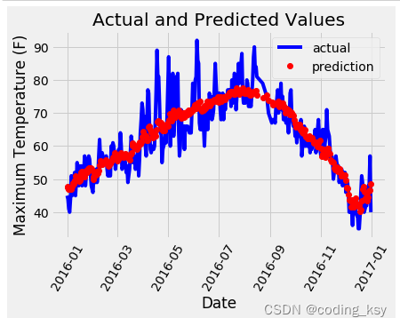
# 真实值
plt.plot(true_data['date'], true_data['actual'], 'b-', label = 'actual')

# 预测值
plt.plot(predictions_data['date'], predictions_data['prediction'], 'ro', label = 'prediction')
plt.xticks(rotation = '60'); 
plt.legend()

# 图名
plt.xlabel('Date'); plt.ylabel('Maximum Temperature (F)'); plt.title('Actual and Predicted Values');