Introducción al principio del algoritmo GAT y análisis del código fuente
Directorio de artículos
Cero. Prólogo (Irrelevante para el texto principal, por favor ignore)
Un breve resumen de los artículos que he analizado antes:
- Conceptos básicos de aprendizaje automático: LR / LibFM
- Intersección de funciones: DCN / PNN / DeepMCP / xDeepFM / FiBiNet / AFM
- Modelado del comportamiento del usuario: DSIN / DMR / DMIN
- Modelado multitarea: MMOE
- Modelado de gráficos: GraphSage
Amplia publicidad
Puede buscar "Jenny's Algorithm Road" o "world4458" en WeChat y seguir mi cuenta pública de WeChat; además, puede leer la columna de Zhihu PoorMemory-Machine Learning, y los artículos futuros también se publicarán en la columna de Zhihu. Siga leyendo CSDN La experiencia será mejor, la dirección es: https://blog.csdn.net/eric_1993/category_9900024.html
1. Información del artículo
- Título del artículo: Gráfico de redes de atención
- Dirección en papel: https://arxiv.org/pdf/1710.10903.pdf
- Dirección del código: https://github.com/PetarV-/GAT
- Publicado: ICLR 2018
- Autor del artículo: ver el artículo para más detalles
- Afiliación del autor: Universidad de Cambridge
2. Ideas centrales
GAT (Graph Attention Networks) utiliza el mecanismo de atención para conocer el peso de los nodos vecinos y obtiene la expresión del propio nodo ponderando y sumando los nodos vecinos.
3. Interpretación de puntos de vista centrales
El mecanismo de implementación de GAT se muestra en la siguiente figura:
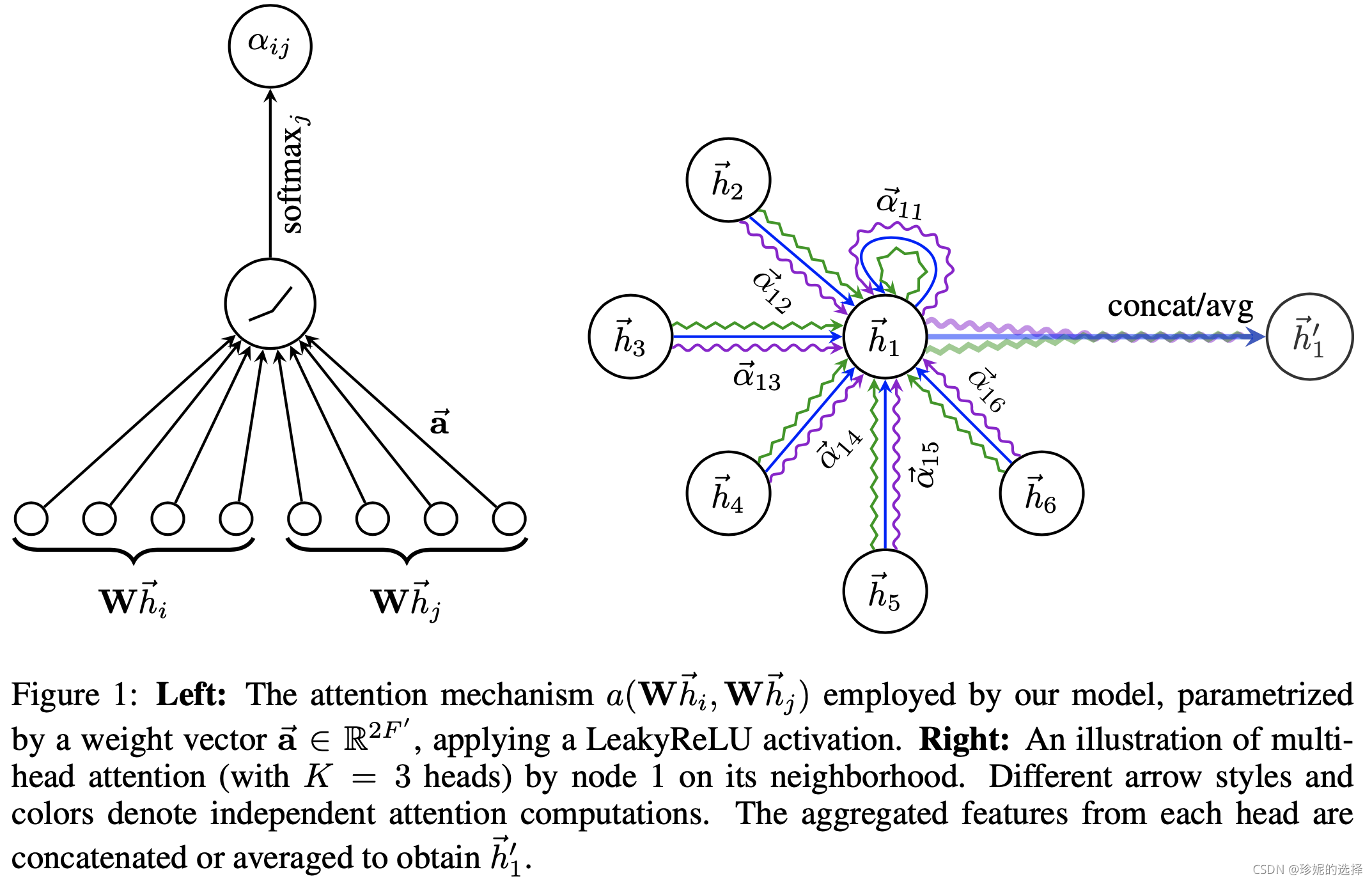
Tenga en cuenta que en la figura de la derecha, GAT adopta Atención de múltiples cabezas, y hay 3 curvas de color en la figura, que representan 3 cabezas diferentes. Bajo diferentes cabezas, el nodo h ⃗ 1 \vec{h}_ {1}h1Puede aprender diferentes incrustaciones y luego combinar/promediar estas incrustaciones para generar h ⃗ 1 ′ \vec{h}_{1}^{\prime}h1′′.
Veamos directamente el código de análisis.
4. Análisis del código fuente
El código fuente de GAT se encuentra en: https://github.com/PetarV-/GAT
La red GAT en sí está formada por el apilamiento de múltiples capas de atención gráfica.Primero, se presenta la implementación de la capa de atención gráfica.
4.1 Capa de atención del gráfico
Definición de la capa de atención del gráfico:
Sea NNLas características de N nodos de entrada son:h = { h ⃗ 1 , h ⃗ 2 , ... , h ⃗ N } , h ⃗ i ∈ RF \mathbf{h}=\left\{\vec{h}_{1} , \vec{h}_{2}, \ldots, \vec{h}_{N}\right\}, \vec{h}_{i} \in \mathbb{R}^{F}h={ h1,h2,…,hnorte},hyo∈RF , usando el mecanismo Atención para generar nuevas características de nodoh ′ = { h ⃗ 1 ′ , h ⃗ 2 ′ , … , h ⃗ N ′ } , h ⃗ i ′ ∈ RF ′ \mathbf{h}^{\prime} = \left\{\vec{h}_{1}^{\prime}, \vec{h}_{2}^{\prime}, \ldots, \vec{h}_{N}^{\ primo }\right\}, \vec{h}_{i}^{\prime} \in \mathbb{R}^{F^{\prime}}h′={ h1′′,h2′′,…,hnorte′′},hi′′∈RF' como salida.
Los coeficientes de atención se generan de la siguiente manera:
α ij = exp ( LeakyReLU ( un → T [ W h ⃗ yo ∥ W h ⃗ j ] ) ) ∑ k ∈ norte yo exp ( LeakyReLU ( un → T [ W h ⃗ yo ∥ W h ⃗ k ] ) ) \alpha_{ij}=\frac{\exp \left(\operatorname{LeakyReLU}\left(\overrightarrow{\mathbf{a}}^{T}\left[\mathbf{W} \vec{h} _{i} \| \mathbf{W} \vec{h}_{j}\right]\right)\right)}{\sum_{k \in \mathcal{N}_{i}} \exp \ left(\operatorname{LeakyReLU}\left(\overrightarrow{\mathbf{a}}^{T}\left[\mathbf{W} \vec{h}_{i} \| \mathbf{W} \vec{ h}_{k}\derecho]\derecho)\derecho)}ayo j=∑k ∈ norteyoExp( L e a k y R e L U(aT[ Whyo∥ Whk] ) )Exp( L e a k y R e L U(aT[ Whyo∥ Whj] ) )
Para a → ∈ R 2 F ′ \overrightarrow{\mathbf{a}} \in \mathbb{R}^{2 F^{\prime}}a∈R2F _′ , mientras que∥ \|∥ significa operación de concatenación.
Su implementación de código se encuentra en: https://github.com/PetarV-/GAT/blob/master/utils/layers.py Tenga en cuenta que en la implementación del código, el método de escritura del autor es muy conciso y sutil, no está escrito directamente según la fórmula anterior, pero con un ligero grado de transformación.
由于a → ∈ R 2 F ′ \overrightarrow{\mathbf{a}} \in \mathbb{R}^{2 F^{\prime}}a∈R2F _′ , 因此令a → = [ a → 1 , a → 2 ] \overrightarrow{\mathbf{a}} = [ \overrightarrow{\mathbf{a}}_{1}, \overrightarrow{\mathbf{a}} _ {2}]a=[a1,a2] , ya → 1 ∈ RF ′ , a → 2 ∈ RF ′ \overrightarrow{\mathbf{a}}_{1}\in\mathbb{R}^{F^{\prime}}, \overrightarrow{\ mathbf{a}}_{2}\in\mathbb{R}^{F^{\prime}}a1∈RF′ ,a2∈RF′ , 那么a → T [ W h ⃗ yo ∥ W h ⃗ j ] \overrightarrow{\mathbf{a}}^{T}\left[\mathbf{W} \vec{h}_{i} \| \mathbf{W} \vec{h}_{j}\right]aT[ Whyo∥ Whj]其实等效于a → 1 TW h ⃗ i + a → 2 TW h ⃗ j \overrightarrow{\mathbf{a}}_{1}^T\mathbf{W}\vec{h}_{i} + \overrightarrow{\mathbf{a}}_{2}^T\mathbf{W}\vec{h}_{j}a1TWhyo+a2TWhj, en la siguiente implementación de código, se adopta el método de escritura equivalente.
def attn_head(seq, out_sz, bias_mat, activation, in_drop=0.0, coef_drop=0.0, residual=False):
	"""
	参数介绍:
	+ seq: 输入节点特征, 大小为 [B, N, E], 其中 N 表示节点个数, E 表示输入特征的大小
	+ out_sz: 输出节点的特征大小, 我这里假设为 H
	+ bias_mat: 做 Attention 时一般需要 mask, 比如只对邻居节点做 Attention 而不包括 Graph 中其他节点.
			它的大小为 [B, N, N], bias_mat 的生成方式将在下面介绍
	+ 其余参数略.

	attn_head 输入大小为 [B, N, E], 输出大小为 [B, N, out_sz]
	"""
    with tf.name_scope('my_attn'):
        if in_drop != 0.0:
            seq = tf.nn.dropout(seq, 1.0 - in_drop)

        ## conv1d 的参数含义依次为: inputs, filters, kernel_size
        ## seq: 大小为 [B, N, E], 经过 conv1d 的处理后, 将得到
        ## 大小为 [B, N, H] 的输出 seq_fts (H 表示 out_sz)
        ## 这一步就是公式中对输入特征做线性变化 (W x h)
        ## seq_fts 就是节点经映射后的输出特征
        seq_fts = tf.layers.conv1d(seq, out_sz, 1, use_bias=False)

        ## f_1 和 f_2 就是我在上面介绍过的, 将向量 a 拆成 a1 和 a2, 然后分别和输入特征进行内积
        ## 再利用 f_1 + tf.transpose(f_2, [0, 2, 1])
        ## 得到每个节点相对其他节点的权重, logits 的大小为 [B, N, N]
        f_1 = tf.layers.conv1d(seq_fts, 1, 1)  ## [B, N, 1]
        f_2 = tf.layers.conv1d(seq_fts, 1, 1)  ## [B, N, 1]
        logits = f_1 + tf.transpose(f_2, [0, 2, 1]) ## [B, N, N]


        ## 将 logits 经过 softmax 前, 还需要加上 bias_mat, 大小为 [B, N, N], 可以认为它就是个 mask,
        ## 对于每个节点, 它邻居节点在 bias_mat 中的值为 0, 而非邻居节点在 bias_mat 中的值为一个很大的负数,
        ## 代码中设置为 -1e9, 这样在求 softmax 时, 非邻居节点对应的权重值就会近似于 0
        coefs = tf.nn.softmax(tf.nn.leaky_relu(logits) + bias_mat)

        if coef_drop != 0.0:
            coefs = tf.nn.dropout(coefs, 1.0 - coef_drop)
        if in_drop != 0.0:
            seq_fts = tf.nn.dropout(seq_fts, 1.0 - in_drop)

        ## coefs 大小为 [B, N, N], 表示每个节点相对于它邻居节点的 Attention 系数,
        ## seq_fts 大小为 [B, N, H], 表示每个节点经变换后的特征
        ## 最后得到 ret 大小为 [B, N, H]
        vals = tf.matmul(coefs, seq_fts)
        ret = tf.contrib.layers.bias_add(vals)

        # residual connection
        if residual:
            if seq.shape[-1] != ret.shape[-1]:
                ret = ret + conv1d(seq, ret.shape[-1], 1)
            else:
                ret = ret + seq

        return activation(ret)  # activation
Aquí hay dos puntos más: conv1dla realización de bias_maty la generación de Primero mire conv1dla realización de:

Veamos la generación bias_matde , el código se encuentra en: https://github.com/PetarV-/GAT/blob/master/utils/process.py , la implementación es la siguiente:
def adj_to_bias(adj, sizes, nhood=1):
	"""
	输入参数介绍:
	+ adj: 大小为 [B, N, N] 的邻接矩阵
	+ sizes: 节点个数, [N]
	+ nhood: 设置多跳, 如果 nhood=1, 则只考虑节点的直接邻居; nhood=2 则把二跳邻居也考虑进去
	"""
    nb_graphs = adj.shape[0]
    mt = np.empty(adj.shape)
    for g in range(nb_graphs):
        mt[g] = np.eye(adj.shape[1])
        ## 考虑多跳邻居的关系, 比如 nhood=2, 则把二跳邻居的关系考虑进去, 之后在 Graph Attention Layer 中,
        ## 计算权重系数时, 也会让二跳邻居参与计算.
        for _ in range(nhood):
            mt[g] = np.matmul(mt[g], (adj[g] + np.eye(adj.shape[1])))

        ## 如果两个节点有链接, 那么设置相应位置的值为 1
        for i in range(sizes[g]):
            for j in range(sizes[g]):
                if mt[g][i][j] > 0.0:
                    mt[g][i][j] = 1.0

    ## 最后返回上面 attn_head 函数中用到的 bias_mat 矩阵,
    ## 对于没有链接的节点位置, 设置一个较大的负数 -1e9; 而有链接的位置, 元素为 0
    ## 这样相当于 mask, 用于 Attention 系数的计算
    return -1e9 * (1.0 - mt)
4.2 Red GAT
El código se define en: https://github.com/PetarV-/GAT/blob/master/models/gat.py , la implementación es la siguiente:
class GAT(BaseGAttN):
    def inference(inputs, nb_classes, nb_nodes, training, attn_drop, ffd_drop,
            bias_mat, hid_units, n_heads, activation=tf.nn.elu, residual=False):
    	"""
    	inputs: 大小为 [B, N, E]
		n_heads: 输入为 [8, 1], n_heads[0]=8 表示使用 8 个 Head 处理输出特征, n_heads[-1]=1, 使用 1 个 Head 处理输出特征
    	"""
        attns = []
        for _ in range(n_heads[0]):
        	## attn_head 的输出大小为 [B, N, H]
            attns.append(layers.attn_head(inputs, bias_mat=bias_mat,
                out_sz=hid_units[0], activation=activation,
                in_drop=ffd_drop, coef_drop=attn_drop, residual=False))
        h_1 = tf.concat(attns, axis=-1)

        ## 重复以上过程
        for i in range(1, len(hid_units)):
            h_old = h_1
            attns = []
            for _ in range(n_heads[i]):
                attns.append(layers.attn_head(h_1, bias_mat=bias_mat,
                    out_sz=hid_units[i], activation=activation,
                    in_drop=ffd_drop, coef_drop=attn_drop, residual=residual))
            h_1 = tf.concat(attns, axis=-1)

        ## 得到输出
        out = []
        for i in range(n_heads[-1]):
            out.append(layers.attn_head(h_1, bias_mat=bias_mat,
                out_sz=nb_classes, activation=lambda x: x,
                in_drop=ffd_drop, coef_drop=attn_drop, residual=False))
        logits = tf.add_n(out) / n_heads[-1]

        return logits
El contenido principal es apilar la capa de atención gráfica, por lo que no lo presentaré en detalle.
V. Resumen
No hay resumen, solo enredo en el corazón.