2.1 Experience with the over-fitting error
Error rate: proportion of sub-sample error
Accuracy: the proportion of the sample points, and the error rate is complementary.
Error: difference between the real output and the predicted output samples. Error learning in the training set is called a training error or experience errors, errors in the new sample called generalization error.
Since the characteristics of the new sample did not know in advance, we can only strive to make the experience error is minimized; although often able to do on the training set classification error rate is zero, but such learning is in most cases not good
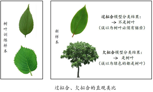
Overfitting: learner learning the training samples of "good", the characteristics of the training sample itself as the general nature of all samples, resulting in generalization performance degradation;
. Solution: 1 optimization goals plus regular items; 2.early stop;
Underfitting: There is no good study of the general nature of the training samples
. Solution: 1 decision tree: expand the branch; 2. neural network: increase the number of training wheels; specific performance as shown below:
2.2 Evaluation
Premise: the real task in terms of generalization performance factors often have a learner, time overhead, storage costs, interpretability assess and make a choice.
We assume an independent test set samples obtained from the true distribution of the sample, the "test error" on the test set as a generalization error of approximation, so the test set and the training set of samples to be mutually exclusive as possible. M samples will generally comprise a data set into a training set and a test set T S, the following are several common methods:
Distillation method:

Cross validation:
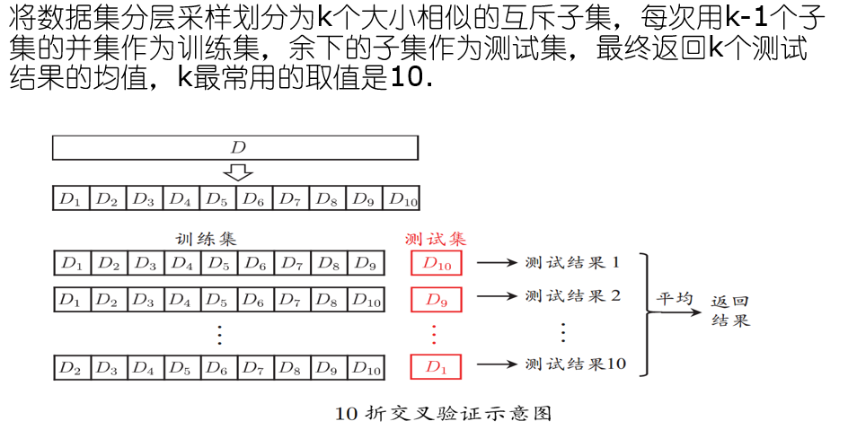

Leave-one, which means that each sample would have become an independent subset, so take a leave all the rest of the way is a leave-one.
Bootstrap:
Explain the source of about one-third probability:
![]()
Where m corresponds to the number N mentioned above, the sampling without replacement every N samples, taking the limit is not able to get the final sample in the limit even if the above expression.
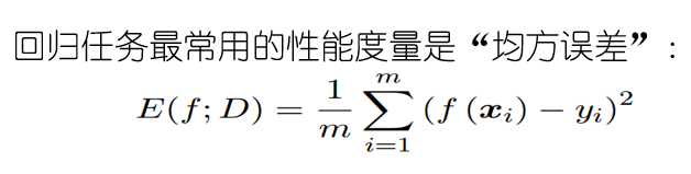
2.3 Performance Measurement
2.3.1 Definition: generalization learner performance be assessed not only feasible and effective test method also requires a measure of evaluation criteria model generalization ability, this evaluation criteria is performance metrics.
Given the sample collection:  wherein Y I is an example of X I real mark, our goal is to learn the prediction result is f (x) is compared with the real marker y.
2.3.2 precision and recall:
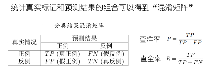
其中TP的意思是True Positive ,FN是Flase Negative,其余的类推。(混淆矩阵请自行百度)
查准率P的意思是在预测结果中挑到真确的比例,类似于小圈子里面的内推,这样P、R的意思就很容易理解了。而后根据学习器的预测结果按正例可能性大小对样例进行排序,并逐个把样本作为正例进行预测,则可以得到查准率-查全率曲线,简称“P-R曲线”
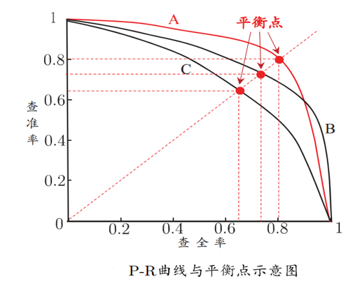
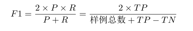
平衡点(BEP)是曲线上“查准率=查全率”时的取值,可用来用于度量P-R曲线有交叉的分类器性能高低,我们的主观当然是P和R越大越好,所以说若一个曲线能被另一个完全包住则说明被包住的性能没有外面的优越,比如优越性能排行:A>B>C,在很多情况下,一般是比较P-R曲线的面积来判断优越性,面积越大则越好。但是这个面积值又不太容易估算,我们就选择平衡点的值来进行比较,值越大越好。但是BEP又过于简单了,于是采用F1度量:
采用调和平均的定义:
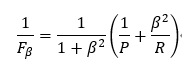
F1即把角标贝塔等于1即可,通过化简:
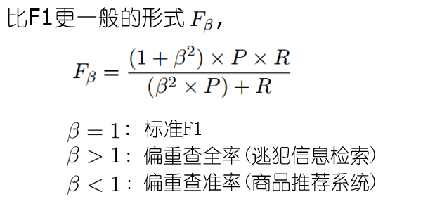
在西瓜书上还有宏的查准率和查全率的概念,其实就是取了一个平均罢了。这里就不急于赘述了,有兴趣可以自行看书。
2.3.3ROC与AUC
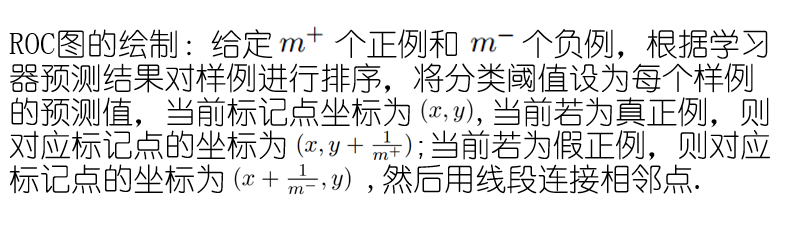
定义:类似P-R曲线,根据学习器的预测结果对样例排序,并逐个作为正例进行预测,以“假正例率”为横轴,“真正例率”为纵轴,可得到ROC曲线,全称“受试者工作特征”.
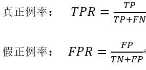
其中ROC图的绘制步骤如下:
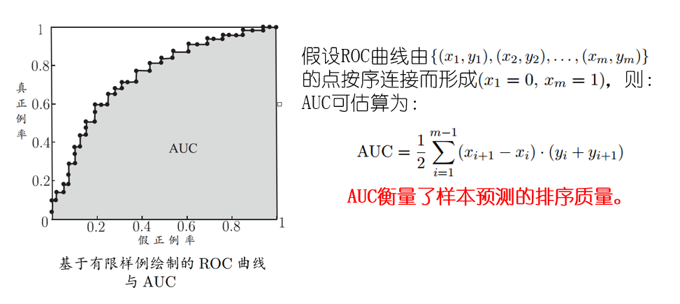
AUC:即ROC下的面积:
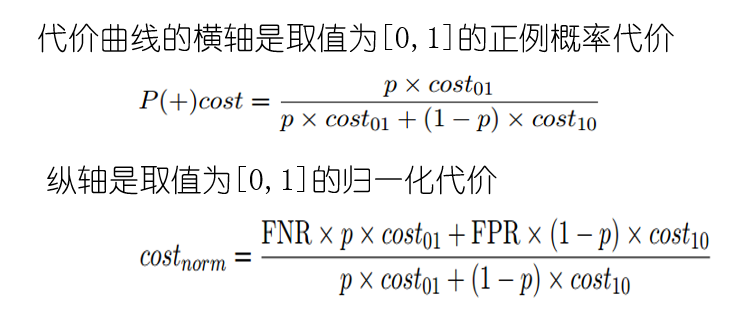
2.3.4代价敏感错误率与代价曲线:
背景:现实任务中不同类型的错误所造成的后果很可能不同,为了权衡不同类型错误所造成的不同损失,可为错误赋予“非均等代价”。
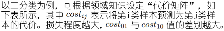
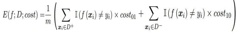
在非均等代价下,不再最小化错误次数,而是最小化“总体代价”,则“代价敏感”错误率相应的为:
在非均等代价下,ROC曲线不能直接反映出学习器的期望总体代价,而“代价曲线”可以。代价曲线的解释如下:
绘制方法:

2.4比较检验
由于测试性能并不等于泛化性能,测试性能随测试集的变化而变化,而且很多机器学习算法具有一定的随机性。直接选取的评估方法往往与现实不太贴切。假设检验为学习器性能比较提供了重要依据。
2.4.1 二项检验

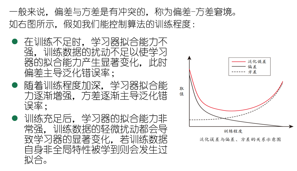
同样,还有 t 检验以及交叉验证 t 检验、McNemar检验、Friedman检验、Nemynyi后续检验、最后再将一个偏差与方差,这个没什么好讲的老套公式,这里给出一个前两个与泛化性能的关系图:
3 阅读材料