Matplotlib
I. acquaintance Matplotlib
Matplotlib Python is an open source graphics library that generates publication-quality graphics in various levels of hardcopy formats and interactive cross-platform environment. By Matplotlib, developers can require only a few lines of code, can generate the drawing, histogram, power spectrum, scatter. Which is a set of function calls matplotlib.pyplot a command-style, which makes matplotlib work together and MATLAB is very similar. Each function pyplo he calls the different functions, for example: a create a point, a point is added to each tag, how the dots, how to create a pattern, to create a drawing area in a drawing, in drawing area Some draw the line, using a modified label graphics.
Second basic usage
drawing (1) of the basic function of the image
data created by a random numpy module, the plot matplotlib library call () method, the basic drawing functions:
Import matplotlib.pyplot AS PLT
Import numpy NP AS
# 1 to 50 -1 point
X = np.linspace (-1,1,20)
Y 2 = X + 1
plt.plot (X, Y)
plt.show ()
Y = 2x + 1de function of the image shown in Figure 1:
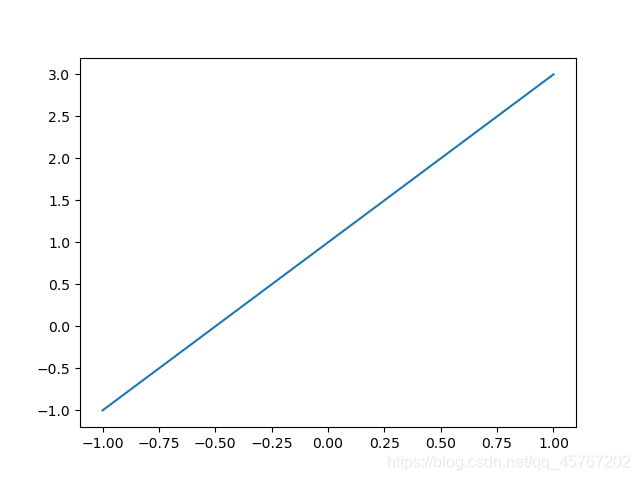
Figure 1
( 2) figure image Introduction
the main function is to set the figure window, how to create more than one-off figure: here by calling the figure at facecolor function, you can set the color of the window frame, while drawing images of the two functions in the same plane.
matplotlib.pyplot AS PLT Import
Import numpy AS NP
X = np.linspace (-1,1,20)
Y1 = 2 X 2 +
Y2 = 2 X ** 2
plt.figure (NUM =. 1, facecolor = "Red")
plt.plot (X, Y1)
plt.figure (2)
plt.plot (X, Y2)
plt.show () 
Plot () command is a versatile, capable of receiving any number of parameters, the same figure how the interface draw multiple images, here we only need to call at a certain figure plt, where we can set the color of the line, there is a difference between the color of the border.
matplotlib.pyplot AS PLT Import
Import numpy AS NP
X = np.linspace (-1,1,20)
Y1 = 2 X 2 +
Y2 = 2 X ** 2
plt.figure (NUM =. 1, facecolor = "Red")
plt.plot (X, Y1)
plt.figure (2)
plt.plot (X, Y1, Color = 'Orange')
plt.plot (X, Y2, Color = 'Pink', lineStyle = '-')
PLT. show ()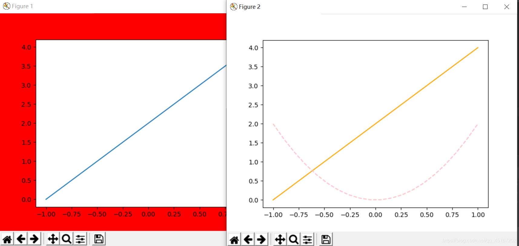
(3) disposed XY axes interesting
plt.xlim ((0,8))
plt.ylim ((- l, 7))
tag #xy axis
plt.xlabel ( 'Axim-X')
plt.ylabel ( 'Y -axim ')
plt.xticks ()
# tag data point meaning
plt.yticks ([0,2,4,7], [' Small ',' alittle ',' Big ',' MOUT '])
plt.show () 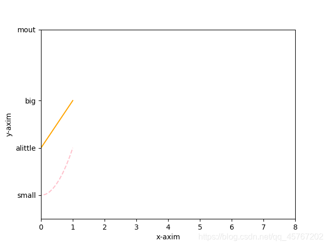
(. 4) is provided Legend Legend
Legend Legend generally applies a function to the plurality of lines indicated the physical meaning, such as is assumed here that the following two functions are represented by the physical meaning of a chicken farm, the number of changes have pigs, how clear score distinguish chickens and pigs have the number, in addition to the label marked on the line segment, the other method is better Legend Legend:
after #L, No. spaced
L1, plt.plot = (X, Y1)
L2, PLT = .plot (X, Y2, Color = 'Pink', lineStyle = '-')
# LOC = Best, Upper right, left Upper, Lower left, Lower right, right, left Center
label and position # map
plt.legend ( = Handles [L1, L2], Labels = [ 'Pig', 'Chicken'], LOC = 'Lower right')
plt.show () 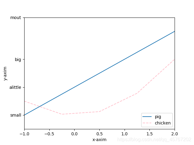
draw (5) images of all
functions described:
plt.plot (x, y, fmt, ...) plotted graph
plt.boxplot (data, notch, position) to draw a box in FIG
plt.bar (left, height, width, bottom) to draw a bar graph
plt.barh (width, bottom, left, height ) Horizontal bar
plt.polar (thera, r) polar diagram
plt.pie (data, explode) pie
plt.psd (x, NFFT = 256, pad_to, Fs) power spectrum FIG density
plt.specgram (x, NFFT = 256, pad_to, F) spectrum
plt.cohere (x, y, NFFT = 256, Fs) XY correlation function
plt.scatter (x, y) scatterplot x and y are the same length
plt.step (x, y, where) the step of FIG order
plt.hist (x, bins, normed) histogram
plt.contour (X, Y, Z, N) equivalent FIG
plt.vlines () vertical Figure
plt.stem (x, y, linefmt, marketfmt) firewood map
plt.plot_date () data date
# pie chart showing the percentage of occupied easy to various types of data, such as the ratio of the number of students universities all grades:
Import matplotlib.pyplot AS plt
labels = 'Freshman', 'Sophomore ', 'junior', 'senior' # custom label
sizes = [22, 26, 28 , 24] # Per a proportion
colors = [ 'yellowgreen', ' gold', 'lightskyblue', 'lightcoral'] # for each block of color
explode = (0, 0.1, 0 , 0) # highlighted third block
plt.pie (sizes, explode = explode, labels = labels, colors = colors, autopct = '% 1.1f% % ', Shadow = True, startAngle = 90)
plt.axis (' equal ') # displayed as a circle, oval avoid compression ratio
plt.sh
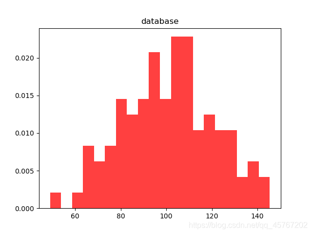
shown below: 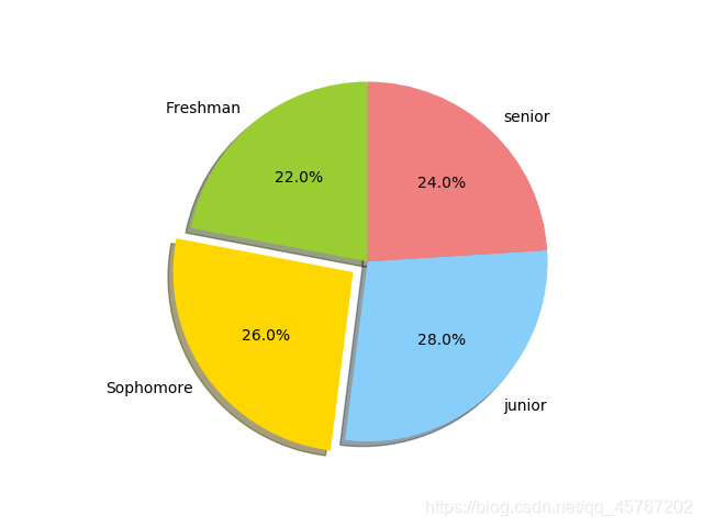 ## histogram:
Import numpy aS NP
Import matplotlib.pyplot aS PLT
np.random.seed (0)
MU, Sigma = 100, mean and standard deviation # 20 is
A = np.random.normal (MU, Sigma, size = 100)
plt.hist (histtype A, 20 is, Density =. 1, = 'stepfilled', facecolor = 'R & lt', Alpha = 0.75)
# 20 which is the number of histogram bins representative of
a normal = 0, indicating the occurrence of height; # normed = 1, the number 1 is the normalized total occurred number
plt.title ( 'Database')
plt.show ()
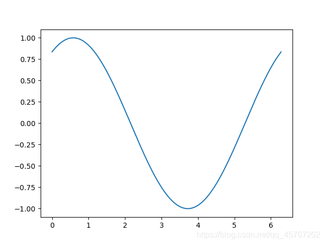
#animation animation
function dynamic animation facilitate analysis of the characteristics of a periodic function, it may exhibit a monotonic function of the dynamic visual characteristics in different sections, following to a sinusoidal function Example:
Import numpy AS NP
Import matplotlib.pyplot AS PLT
# animation module
from matplotlib Import animation
Fig, AX = plt.subplots ()
X = np.arange (0,2 np.pi, 0.01)
Line, = ax.plot (X, np.sin (X))
# update mode, loop
DEF Animate (I):
line.set_ydata (np.sin (I + X / 100))
return Line,
DEF the init ():
line.set_ydata (NP .sin (X))
return Line,
# label, length, number of frames, long interval,
ANI = animation.FuncAnimation (Fig = Fig, FUNC = Animate, frames = 100, the init = init_func, interval The = 20 is, the blit = False )
plt.show ()
III. summary
matplolib module simple and convenient solution to the problem of image intuitive mathematics and drawing, worth serious study.
