Boosting algorithm
Boosting is an algorithm used to improve the accuracy of weak classifiers, is the "weak learning algorithm" to the "strong learning algorithm" process, the main idea is to "Three Stooges top one Zhuge Liang." In general, a weak learning algorithm to find relatively easy, then get a series of weak classifiers through repeated study, the combination of weak classifiers to get a strong classifier.
Boosting algorithm to involve two parts, and the additive model algorithm to the front step.
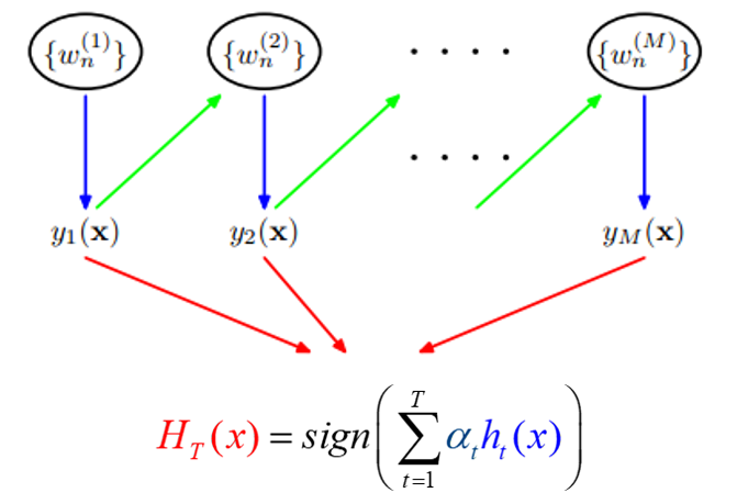
Additive model that is obtained by adding a strong classifier by a series of linear weak classifiers. Usually the following combination:
$$ F_M (X; P) = \ sum_. 1} ^ {n-m = \ beta_mh (X; a_m) $$
wherein, $ h (x; a_m) $ is one of the weak classifiers, $ a_m $ is weak classifiers to learn the optimal parameters, $ \ beta_m $ is weak classifier learning in strong proportion, $ P $ are all combinations of $ \ alpha_m $ and $ \ beta_m $ a. These weak classifiers strong classifier consisting of linear addition.
Former iterations to generate a classifier that is a step in the training process, the next round of training is come in the last round basis. I.e. can be written in this form:
$$ F_m (X) = F_ {}. 1-m (X) + \ beta_mh_m (X; a_m) $$
With the following GIF will look more vivid

The basic concept Adaboost
AdaBoost is a typical Boosting algorithm, belongs to a family of Boosting.

For AdaBoost, we have to figure out two things:
1, each iteration of weak learning $ h (x; a_m) $ What is not the same, how to learn?
2, the weak classifier weights $ \ beta_m $ How to determine?
The first question, AdaBoost approach is to enhance those rights were wrongly classified samples of the previous round of weak classifiers value, while reducing those rights were correctly classified sample values. As a result, those who do not get proper data classification, due to its weight increase and subject to greater attention after another round of weak classifiers. Thus, the classification by a series of weak classifiers "divide and rule."
第二个问题,即弱分类器的组合,AdaBoost采取加权多数表决的方法。具体地,加大分类误差率小的弱分类器的权值,使其在表决中起较大的作用,减小分类误差率大的弱分类器的权值,使其在表决中起较小的作用。
Adaboost算法流程-分类
输入:训练数据集$T={(x_1,y_1),(x_2,y_2),...,(x_N,y_N)}$,其中,$x_i∈X?R^n$,$y_i∈Y={-1,1}$,迭代次数$M$
1.初始化训练样本的权值分布:
$$
\begin{aligned}
D_1=(w_{1,1},w_{1,2},…,w_{1,i}),\w_{1,i}=\frac{1}{N},i=1,2,…,N
\end{aligned}
$$
2.对于$m=1,2,…,M$
(a) 使用具有权值分布$D_m$的训练数据集进行学习,得到弱分类器$G_m (x)$
(b) 计算$G_m(x)$在训练数据集上的分类误差率:$$e_m=\sum_{i=1}^Nw_{m,i} I(G_m (x_i )≠y_i )$$
(c) 计算$G_m (x)$在强分类器中所占的权重:$$\alpha_m=\frac{1}{2}log \frac{1-e_m}{e_m} $$
(d) 更新训练数据集的权值分布(这里,(z_m)是归一化因子,为了使样本的概率分布和为1):
$$w_{m+1,i}=\frac{w_{m,i}}{z_m}exp?(-\alpha_m y_i G_m (x_i )),i=1,2,…,10$$
$$z_m=\sum_{i=1}^Nw_{m,i}exp?(-\alpha_m y_i G_m (x_i ))$$
3.得到最终分类器:
$$F(x)=sign(\sum_{i=1}^N\alpha_m G_m (x))$$
公式推导
假设已经经过$m-1$轮迭代,得到$F_{m-1} (x)$,根据前向分步,我们可以得到:
$$F_m (x)=F_{m-1} (x)+\alpha_m G_m (x)$$
我们已经知道AdaBoost是采用指数损失,由此可以得到损失函数:
$$
\begin{aligned}
Loss=&\sum_{i=1}^Nexp?(-y_i F_m (x_i ))\
=&\sum_{i=1}^Nexp?(-y_i (F_{m-1} (x_i )+\alpha_m G_m (x_i )))
\end{aligned}
$$
这时候,$F_{m-1}(x)$是已知的,可以作为常量移到前面去:
$$Loss=\sum_{i=1}^N\widetilde{w_{m,i}} exp?(-y_i \alpha_m G_m (x_i ))$$
其中,$\widetilde{w_{m,i}}=exp?(-y_i (F_{m-1} (x)))$ 就是每轮迭代的样本权重!依赖于前一轮的迭代重分配。
再化简一下:
$$
\begin{aligned}
\widetilde{w_{m,i}}=&exp?(-y_i (F_{m-1} (x_i )+\alpha_{m-1} G_{m-1} (x_i )))\=&\widetilde{w_{m-1,i}} exp?(-y_i \alpha_{m-1} G_{m-1} (x_i ))
\end{aligned}
$$
继续化简Loss:
$$
\begin{aligned}
Loss=\sum_{y_i=G_m(x_i)}\widetilde{w_{m,i}} exp(-\alpha_m)+\sum_{y_i≠G_m(x_i)}\widetilde{w_{m,i}} exp?(\alpha_m)\=\sum_{i=1}^N\widetilde{w_{m,i}}(\frac{\sum_{y_i=G_m(x_i)}\widetilde{w_{m,i}}}{\sum_{i=1}^N\widetilde{w_{m,i}}}exp(-\alpha_m)+\frac{\sum_{y_i≠G_m(x_i)}\widetilde{w_{m,i}}}{\sum_{i=1}^N\widetilde{w_{m,i}}}exp(\alpha_m))
\end{aligned}
$$
其中
$\frac{\sum_{y_i≠G_m(x_i)}\widetilde{w_{m,i}}}{\sum_{i=1}^N\widetilde{w_{m,i}}}$就是分类误差率$e_m$
所以
$Loss=\sum_{i=1}^N\widetilde{w_{m,i}}exp?(-\alpha_m)+e_m exp?(\alpha_m))$
这样我们就得到了化简之后的损失函数
对$\alpha_m$求偏导令$\frac{?Loss}{?\alpha_m }=0$得到:
$$\alpha_m=\frac{1}{2}log\frac{1-e_m}{e_m}$$
AdaBoost实例
《统计学习方法》上面有个小例子,可以用来加深印象
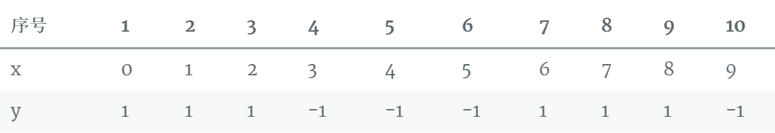
有如下的训练样本,我们需要构建强分类器对其进行分类。x是特征,y是标签。
令权值分布$D_1=(w_{1,1},w_{1,2},…,w_{1,10} )$
假设一开始的权值分布是均匀分布:$w_{1,i}=0.1,i=1,2,…,10$
现在开始训练第一个弱分类器。我们发现阈值取2.5时分类误差率最低,得到弱分类器为:
$$
G_1(x)=
\begin{cases}
1,& \text{x<2.5} \
-1,& \text{x>2.5}
\end{cases}
$$
当然,也可以用别的弱分类器,只要误差率最低即可。这里为了方便,用了分段函数。得到了分类误差率$e_1=0.3$
第二步计算$G_1 (x)$在强分类器中的系数$\alpha_1=\frac{1}{2} log\frac{ 1-e_1}{e_1}=0.4236$
第三步更新样本的权值分布,用于下一轮迭代训练。由公式:
$$w_{2,i}=\frac{w_{1,i}}{z_1}exp?(-\alpha_1 y_i G_1 (x_i )),i=1,2,…,10$$
得到新的权值分布,从各0.1变成了:
$D_2=(0.0715,0.0715,0.0715,0.0715,0.0715,0.0715,0.1666,0.1666,0.1666,0.0715)$
可以看出,被分类正确的样本权值减小了,被错误分类的样本权值提高了。
第四步得到第一轮迭代的强分类器:
$$sign(F_1 (x))=sign(0.4236G_1 (x))$$
以此类推,经过第二轮……第N轮,迭代多次直至得到最终的强分类器。迭代范围可以自己定义,比如限定收敛阈值,分类误差率小于某一个值就停止迭代,比如限定迭代次数,迭代1000次停止。这里数据简单,在第3轮迭代时,得到强分类器:
$$sign(F_3 (x))=sign(0.4236G_1 (x)+0.6496G_2 (x)+0.7514G_3 (x))$$
的分类误差率为0,结束迭代。
$F(x)=sign(F_3 (x))$就是最终的强分类器。
Adaboost参数详解
我们直接使用sklearn.ensemble中的AdaBoostRegressor和AdaBoostClassifier,两者大部分框架参数是相同的:
AdaBoostRegressor
class sklearn.ensemble.AdaBoostRegressor
(base_estimator=None, n_estimators=50,
learning_rate=1.0, loss=’linear’, random_state=None)
AdaBoostClassifier
class sklearn.ensemble.AdaBoostClassifier
(base_estimator=None, n_estimators=50,
learning_rate=1.0, algorithm=’SAMME.R’, random_state=None)
参数
1)base_estimator:AdaBoostClassifier和AdaBoostRegressor都有,即我们的弱分类学习器或者弱回归学习器。理论上可以选择任何一个分类或者回归学习器,不过需要支持样本权重。我们常用的一般是CART决策树或者神经网络MLP。默认是决策树,即AdaBoostClassifier默认使用CART分类树DecisionTreeClassifier,而AdaBoostRegressor默认使用CART回归树DecisionTreeRegressor。另外有一个要注意的点是,如果我们选择的AdaBoostClassifier算法是SAMME.R,则我们的弱分类学习器还需要支持概率预测,也就是在scikit-learn中弱分类学习器对应的预测方法除了predict还需要有predict_proba。
2)algorithm:这个参数只有AdaBoostClassifier有。主要原因是scikit-learn实现了两种Adaboost分类算法,SAMME和SAMME.R。两者的主要区别是弱学习器权重的度量,SAMME使用了二元分类Adaboost算法的扩展,即用对样本集分类效果作为弱学习器权重,而SAMME.R使用了对样本集分类的预测概率大小来作为弱学习器权重。由于SAMME.R使用了概率度量的连续值,迭代一般比SAMME快,因此AdaBoostClassifier的默认算法algorithm的值也是SAMME.R。我们一般使用默认的SAMME.R就够了,但是要注意的是使用了SAMME.R, 则弱分类学习器参数base_estimator必须限制使用支持概率预测的分类器。SAMME算法则没有这个限制。
3)loss:这个参数只有AdaBoostRegressor有,Adaboost.R2算法需要用到。有线性‘linear’, 平方‘square’和指数 ‘exponential’三种选择, 默认是线性,一般使用线性就足够了,除非你怀疑这个参数导致拟合程度不好。
4)n_estimators: AdaBoostClassifier和AdaBoostRegressor都有,就是我们的弱学习器的最大迭代次数,或者说最大的弱学习器的个数。一般来说n_estimators太小,容易欠拟合,n_estimators太大,又容易过拟合,一般选择一个适中的数值。默认是50。在实际调参的过程中,我们常常将n_estimators和下面介绍的参数learning_rate一起考虑。
5)learning_rate: AdaBoostClassifier和AdaBoostRegressor都有,即每个弱学习器的权重缩减系数ν,在原理篇的正则化章节我们也讲到了,加上了正则化项,我们的强学习器的迭代公式为$fk(x)=fk?1(x)+ναkGk(x)$。ν的取值范围为0<ν≤1。对于同样的训练集拟合效果,较小的ν意味着我们需要更多的弱学习器的迭代次数。通常我们用步长和迭代最大次数一起来决定算法的拟合效果。所以这两个参数n_estimators和learning_rate要一起调参。一般来说,可以从一个小一点的ν开始调参,默认是1。
SAMME.R算法流程
1.初始化样本权值:
$$w_i=1/N,i=1,2,…,N$$
2.Repeat for$m=1,2,…,M$
2.1 训练一个弱分类器,得到样本的类别预测概率分布$p_m(x)=P(y=1|x)∈[0,1]$
2.2 $f_m(x)=\frac{1}{2}log\frac{p_m(x)}{1-p_m(x)}$
2.3 $w_i=w_iexp[-y_if_m(x_i)]$,同时,要进行归一化使得权重和为1
3.得到强分类模型:$sign{\sum_{m=1}^{M}f_m(x)}$
DecisionTreeClassifier和DecisionTreeRegressor的弱学习器参数,以CART分类树为例,这里就和前文随机森林类似了。

方法
decision_function(X):返回决策函数值
fit(X,Y):在数据集(X,Y)上训练模型
get_parms():获取模型参数
predict(X):预测数据集X的结果
predict_log_proba(X):预测数据集X的对数概率
predict_proba(X):预测数据集X的概率值
score(X,Y):输出数据集(X,Y)在模型上的准确率
staged_decision_function(X):返回每个基分类器的决策函数值
staged_predict(X):返回每个基分类器的预测数据集X的结果
staged_predict_proba(X):返回每个基分类器的预测数据集X的概率结果
staged_score(X, Y):返回每个基分类器的预测准确率。
Adaboost总结
Adaboost优点
1.可以使用各种方法构造子分类器,Adaboost算法提供的是框架
2.简单,不用做特征筛选
3.相比较于RF,更不用担心过拟合问题
Adaboost缺点
1.从wiki上介绍的来看,adaboost对于噪音数据和异常数据是十分敏感的。Boosting方法本身对噪声点异常点很敏感,因此在每次迭代时候会给噪声点较大的权重,这不是我们系统所期望的。
2.运行速度慢,凡是涉及迭代的基本上都无法采用并行计算,Adaboost是一种"串行"算法.所以GBDT(Gradient Boosting Decision Tree)也非常慢。
参考:
李航《统计学习方法》第8章 提升方法
《Getting Started with Machine Learning》Jim Liang
https://www.cnblogs.com/pinard/p/6136914.html
https://www.cnblogs.com/ScorpioLu/p/8295990.html
https://louisscorpio.github.io/2017/11/28/AdaBoost入门详解/
https://ask.hellobi.com/blog/zhangjunhong0428/10361
本文由博客一文多发平台 OpenWrite 发布!