Table of contents

1. Equality constrained optimization (eg. llp)

1.2 Qualified sums

2. Inequality constraint optimization (eg. svm)

3. Unconstrained (eg. ls)

1. Gradient descent method

2. Common definitions and properties of traces

4. Kronecker product

synopsis

This blog is used to record various pre-knowledge required for machine learning theory learning and optimization problem derivation.

1. Lagrangian function

In the optimization problem, after the optimization problem and constraints of the method are obtained, the corresponding Lagrangian function is often required and solved. The following is the construction method of the Lagrangian function in several common situations.

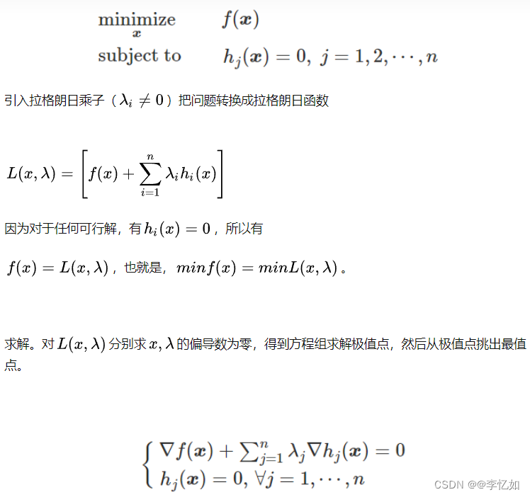
1. Equality constrained optimization (eg. llp)

1.1 No summation

$\large \min _{\mathbf{a}} \mathbf{a}^{T} \mathbf{S a}, \quad \text { s.t. } \mathbf{a}^{T} \mathbf{a}=1$

Define its Lagrangian function as:

$\large L(\mathbf{a}, \lambda)=\mathbf{a}^{T} \mathbf{S a}+\lambda\left(1-\mathbf{a}^{T}\mathbf{a }\right)$

Find the partial derivative for the corresponding unknown (here α)

$\large \mathbf{S a}=\lambda \mathbf{a}$

Then use eigendecomposition to the above formula to solve the original optimization problem.

1.2 Qualified sums

2. Inequality constraint optimization (eg. svm)

$\large \begin{array}{l} \min _{\mathbf{u}} f_{0}(\mathbf{u}) \\ \text { st } f_{i}(\mathbf{u}) \ leq 0, i=1.2, \cdots, n \end{array}$

Define its Lagrangian function as:

$\large L(\mathbf{u}, \boldsymbol{\alpha})=f_{0}(\mathbf{u})+\sum_{i=1}^{n} \alpha_{i} f_{i}(\mathbf{u})$

Find the partial derivative for the corresponding unknown, and set it to 0.

3. Unconstrained (eg. ls)

It directly corresponds to the requirement to solve the unknown to find the partial derivative, and let it be 0.

2. Norm

1. F norm

The F norm is a matrix norm. Assuming that A is an mxn matrix, the corresponding F norm is defined as follows:

$\large \|A\|_{F}=\sqrt{\operatorname{tr}\left(A^{T} A\right)}=\sqrt{\sum_{i, j} a_{i j}^{2}}$

2.l2 norm

The l2 norm is the Euclidean distance, which is often used to measure "error". It is defined as follows:

$\large \|x\|_{2}=\left(\left|\boldsymbol{x}_{1}\right|^{2}+\left|\boldsymbol{x}_{2}\right|^{2}+\cdots+\left|\boldsymbol{x}_{\boldsymbol{n}}\right|^{2}\right)^{1 / 2}$

For matrices, the l2 norm is defined as follows:

$\large \|A\|_{2}=\sqrt{\lambda_{\max }\left(A^{T} A\right)}$

Tips: The parameter is the absolute value of the corresponding maximum eigenvalue.

3.l1 norm

The l1 norm is the sum of absolute values, defined as follows:

$\large \|X\|_{1}=\left(\left|x_{1}\right|+\left|x_{2}\right|+\ldots+\left|x_{n}\right|\right)$

4.l2,1 norm

The l2,1 norm is to first find the l2 norm by column and then find the l1 norm by row, which is defined as follows:

$\large \|W\|_{2,1}=\|w\|_{1}=\sum_{i=1}^{d} \sqrt{\sum_{j=1}^{n}\left|W_{i, j}\right|^{2}}$

Define the corresponding D matrix, l2, 1 norm can be rewritten as:

$\large \|W\|_{2,1}=tr\left ( P^TDP \right )$

where D is a diagonal matrix, and the diagonal is the square of the two-norm of 1/row.

3. Partial guide

The commonly used partial derivative of the trace of the matrix is as follows:

$\large \frac{\partial \operatorname{tr}\left(A^{T} X\right)}{\partial x_{i j}}=\frac{\partial \operatorname{tr}\left(X^{T} A\right)}{\partial x_{i j}}=a_{i j}=[A]_{i j}$

$\large \frac{\partial \operatorname{tr}\left(X^{T} A X\right)}{\partial x_{i j}}=\sum_{q=1}^{m} a_{i q} x_{q j}+\sum_{p=1}^{m} a_{p i} x_{p j}=\left[A X+A^{T} X\right]_{i j}$

For details, please refer to: The relationship between the Frobenius norm of the matrix and the trace (trace) and its partial derivative rule_Love life's blog

Summary and detailed explanation: the trace of the matrix and the derivation of the matrix by the trace

1. Gradient descent method

The gradient descent method is commonly used in iteration and optimization. The calculation formula can be simply understood as finding the corresponding partial derivative, as follows:

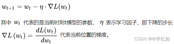
The purpose of gradient descent is to continuously update the weight parameter w, so that the value of the loss function L is continuously reduced.

2. Common definitions and properties of traces

1.tr(AB) = tr(BA)

2.tr(A) = tr(A^T)

3.tr(A + B) = tr(A) + tr(B)

4.tr( rA ) = r tr( A ) = tr(rA * I) (i is the identity matrix)

4. Kronecker product

The Kronecker product is an operation between two matrices of any size, and the result is a matrix, denoted by . The Kronecker product is a special form of the tensor product , as follows:

Introduction to machine learning theory and pre-requisite knowledge

1. Lagrangian function

1. Equality constrained optimization (eg. llp)

1.1 No summation

1.2 Qualified sums

2. Inequality constraint optimization (eg. svm)

3. Unconstrained (eg. ls)

2. Norm

1. F norm

2.l2 norm

3.l1 norm

4.l2,1 norm

3. Partial guide

1. Gradient descent method

2. Common definitions and properties of traces

4. Kronecker product

Guess you like