A. Speaking from the story of the linear regression

I believe we all heard the famous naturalist, Charles Darwin's name, and the hero of today's story is his cousin Galton.

Galton was a physiologist, in 1995, he studied the 1078 heap and his son's height and found that they generally satisfy a formula, that is,

Y = 0.8567 + 0.516 * x

This formula of x refers to the father's height, Y refers to the son's height. It is clear that this is what we learned in high school linear equations, reaction on a plane is a straight line .

By this formula, we might intuitively father will always be there for the tall tall son, the father will have shorter shorter son. But Galton further observed that not all cases are like this. Particularly high father's son will be shorter than his father some special dwarf father's son will be higher than some of his father, said his son would not have continued to go higher or shorter. This phenomenon, in fact, return . Trend will not last forever, but will return to a center.

Through this story, I believe you have to understand what is linear regression, then the next we are concerned that more details.

II. Understanding Linear Regression

Plane coordinate point

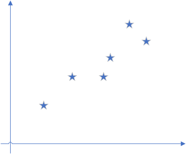
Throws question: Suppose there is such a number of points, which are the available data, we have to find the line fitting these points, and then predict the next point. Then we want to find out how this line on the road?

h (x) = a0 + a1 * x (a1 is the slope, a0 is the intercept)

Or another question is asked, how we want to find a_1 and a_0 it?

Cost Function (cost function)

First contact with the linear regression students may not know what the cost function, in fact, when it comes to the concept of do not know, as long as want to know two things, the concept of what is, what is the use. Think clearly these two points, at least it will not be puzzled.

What is the cost functions are?

Let's just draw two lines to fit those points, as shown, it can be seen clearly Figure II is more fitting to say Figure II line closer to our ideal line.
The cost function introduction

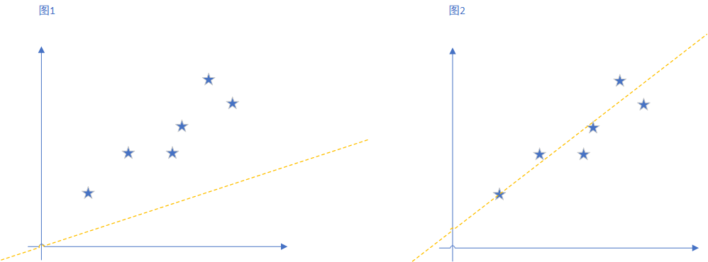
OK, then carefully observed, Figure II line and a line any different? The most obvious is the view of a respective point along the y axis to farther distance piece line, and at various points in Figure II closer to the line distance.
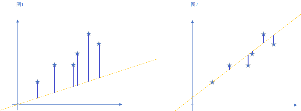
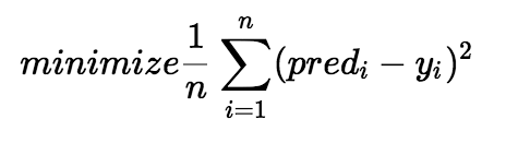
The distance to each point of the west line

This all points along the y axis to the line error, i.e. error of each point, the average value. Is the cost function. Formula is as follows:

The cost function formula

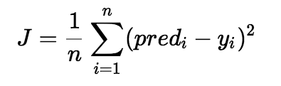
Pred (i) is the i-th point, the value of the line y, y (i) is the i-th point, the y value of a point, is avoided mainly square plus a negative number. This is the cost function.

The cost function What is the use?

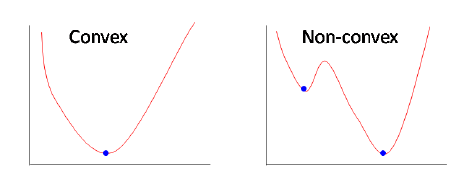
The cost function may help us to find the best values of a0 and a1. As mentioned earlier, the cost function for each point in the y-axis is the average distance between the straight line. Our goal is to minimize the value, in the general case, the cost function is convex, as shown,

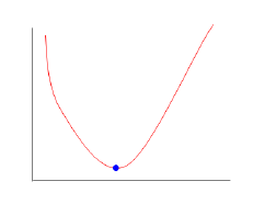
This function is not seeing more familiar? We do not often see such a thing in learning Figure derivative, this chart usually by derivation of the solution.

Minimization process

From y = a0 + a1 * x, this line begins. To write the cost function, our goal has not changed, it is to find a0 and a1, make this line more closely aligns those points (cost function is to make the smallest). Of course, we have not when it comes to how to minimize the cost function, here we then talk about how to make the cost function to minimize it.

Gradient Descent (gradient descent)

What gradient decline was?

Gradient descent is an iterative constantly updated a0 and a1 method of reducing the cost function. We can derivation of the cost function the way it should be seen that let a0 or a1 to add or subtract.

Gradient descent equation
In fact, the upper part of the derivation of the cost function, through its derivation, we can know a0 and a1 should be increased or decreased.

Solving coefficient formula

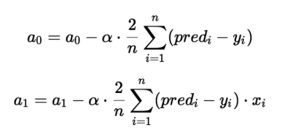
This formula is actually a (partial derivatives a0- cost function). Of course, where there is a rate α (Alpha) control, the derivative of the cost function to know a0 and a1 is increased or decreased, it should be increased [alpha] is much, much reduced.

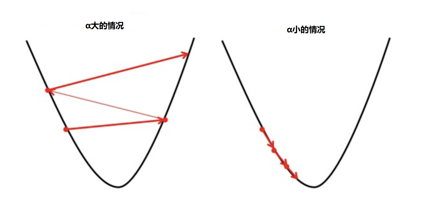
For example, suppose you are now in the semi hillside, you have to do is down, the partial derivatives of the cost function is to tell you to be down or up. Α is the rate controlling step to step much.

Small steps (α small) means small run down the mountain, the disadvantage is the relatively long run. Major step forward (α large) means faster, but may suddenly step too, he ran across the hillside to go.

Rate of action of the α

Gradient descent what's the use?

By gradient descent, so that we can find a0 and a1 a local optimal solution, and why it is locally optimal solution? Examples because the problem may not be a reality in the beginning so clear, many times you may find this line can be, this line is not bad, the piece seems to be. The computer will be so, it may also feel a certain line has been good enough. Do not go to the other line.

Reaction to which we ask questions, we can say because it is a minimization problem (minimizing the cost function), but it might as right as it is already the smallest in a local inside, left to right are increased, since so it is peace of mind when salted fish myself. This phenomenon and the initial random selection, but also on the rate and training related.

Local optimum and global optimum

After selecting an appropriate value of α, sufficient number of times when the iteratively updated. Theoretically it will reach a bottom, which means that when the cost function is within a certain range minimal. This time the a0 a1 drink was seeking us out, we will be able to get a straight line fit of the points in space.

Finally tell you, just introduced only in two-dimensional space are calculated, which is only one feature. But in reality, there is often more than one feature, but a plurality of features, such as the following forms:

h(x)=a0 + a1 * x1 + a2 * x2 + a3 * x3 ...

However, the calculation methods and calculation methods are similar. But the amount of data becomes much more complicated calculations.

OK, start with an example of today began to introduce linear regression. Then the cost function described, as well as a method of solving the cost function is minimized, gradient descent. We will be back on to do a linear regression, and introduce a variety of other preliminary regression analysis using sklearn.

Above ~

Popular have to say a linear regression algorithm (a) linear regression preliminary presentation