Convolutional neural network (Convolutional Neural Network, CNN). Deep Learning is a general term for all deep learning algorithms, CNN application is a deep learning algorithm in image processing field.
Convolution neural network is an efficient identification method developed in recent years, and caused widespread attention. Neuron 1960, Hubel and Wiesel for topical studies in cats and direction sensitive cortex selected found unique network structure can effectively reduce the complexity of the feedback neural network, in turn, presents convolutional neural network (when Convolutional Neural Networks- referred CNN). Now, CNN has become a hot topic of many scientific fields, especially in the field of pattern classification, due to the complexity of the network to avoid the pre-pretreatment on the image, you can directly enter the original image, which has been more widely used. Identifying new machine K.Fukushima proposed in 1980, it was the first to realize the network convolution neural network. Subsequently, more researchers to the network has been improved. Among them, the research results are representative Alexander and Taylor's "improved cognitive machine", which combines the advantages of various improved method avoids the time-consuming and error back propagation.
Generally, the basic CNN structure comprises two layers, one layer of feature extraction, and the input of each neuron is connected to the front layer of the receiving local domain, and extracting the local feature. Once the features are extracted locally, it will determine the positional relationship between the other features and down; second mapping layer wherein each layer is calculated by a plurality of characteristics of the network maps, each map feature is a plane, All weights equal neurons plane. Wherein the mapping structure using the influence function nucleosomes sigmoid function as the activation function convolution of the network, characterized in that the displacement map having invariance. Further, since the weight of neurons share a mapping surface, thus reducing the number of free parameters of the network. Each layer convolution convolutional neural network are followed by a request for the local average is calculated and the secondary layer is extracted twice with this unique structural feature extraction feature resolution is reduced.
Convolution neural network applications
CNN primarily used to identify a displacement, distortion and other forms of scaling invariance two-dimensional pattern. Since the CNN learning feature detection layer by the training data, so when using the CNN, the display characteristic avoids extraction, implicitly learn from the training data; Furthermore since the same feature map neural right side of the same value , so the network can be a parallel study, which is the convolution with respect to a network of neurons connected to each other big advantage of the network. Convolutional neural network weights to its special structure shared with local speech recognition and image processing unique advantages, which is closer to the actual layout of biological neural networks, the weights sharing reduces the complexity of the network, in particular multidimensional image input vector may be directly input network this feature avoids the complexity of the process of feature extraction and classification of the data reconstruction.
Principle convolution neural network
Neural Networks
First introduced neural network, this step can be detailed reference resources 1. Briefly below. Each neural network unit is as follows: 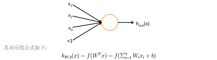 wherein, the unit may also be referred to as a Logistic regression model. When combining a plurality of cells and having a layered structure neural network model is formed. The following figure illustrates a hidden layer having a neural network.
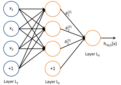
Corresponding to the following formula: 
relatively similar, it can be extended to have a 2,3,4,5, ... a hidden layer. The method of training the neural network with Logistic also similar, but due to its multi-layered nature, also need to use the chain rule for derivation node hidden layer is the derivative, i.e., the gradient descent + chain derivation method, reverse professional name propagation. About training algorithms, this involves temporarily.
Convolution neural network
By Hubel and Wiesel on the physiology of the cat visual cortex electrical inspired, it was suggested convolutional neural network (CNN), Yann Lecun earliest CNN for Digital Recognition and has maintained its dominance in the problem. In recent years, continuous efforts convolution neural networks in multiple directions, speech recognition, face recognition, general object recognition, motion analysis, natural language processing analysis of brain waves even have a breakthrough.
The difference between the ordinary convolutional neural network and the neural network is that the convolutional neural network comprises a feature extractor and a layer composed of a convolution subsampling layer. Convolution layer convolutional neural network, connected to only a part of neurons in adjacent layers of neurons. In one convolution in the CNN layer, typically comprising a number of feature plane (featureMap), each characterized by a number of planar array of rectangular neurons, neurons in the same plane shared feature weights, where the weight is shared volume convolution kernel. Convolution kernel generally in the form of a matrix of random decimal initialization, convolution kernel will learn to get reasonable weights during training network. Direct benefits of shared weights (convolution kernel) bring is to reduce the connection between the network layers, while reducing the risk of over-fitting. Subsampling also called pooled (pooling), subsampling usually mean (mean pooling) and maximum sub-sampling (max pooling) in two forms. Sub-sampling can be seen as a special convolution process. Convolution and subsampling greatly simplifies the complexity of the model, the model parameters is reduced. The basic structure of the convolutional neural network as shown: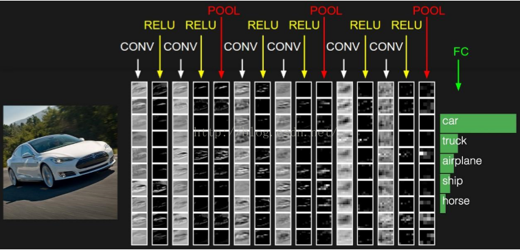
Convolutional neural network consists of three parts. The first part is the input layer. The second part of a combination of layers and the n convolution pooled layers. The third part consists of a full coupling of Multilayer Perceptron classifier configured.
Local receptive field
卷积神经网络有两种神器可以降低参数数目,第一种神器叫做局部感知野。一般认为人对外界的认知是从局部到全局的,而图像的空间联系也是局部的像素联系较为紧密,而距离较远的像素相关性则较弱。因而,每个神经元其实没有必要对全局图像进行感知,只需要对局部进行感知,然后在更高层将局部的信息综合起来就得到了全局的信息。网络部分连通的思想,也是受启发于生物学里面的视觉系统结构。视觉皮层的神经元就是局部接受信息的(即这些神经元只响应某些特定区域的刺激)。如下图所示:左图为全连接,右图为局部连接。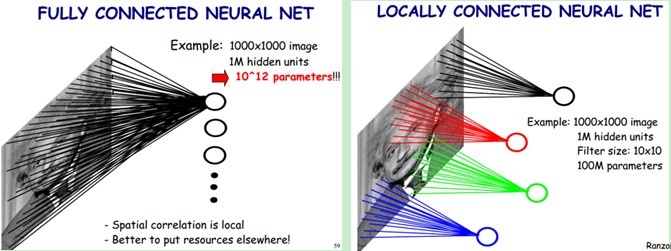
在上右图中,假如每个神经元只和10×10个像素值相连,那么权值数据为1000000×100个参数,减少为原来的万分之一。而那10×10个像素值对应的10×10个参数,其实就相当于卷积操作。
权值共享
但其实这样的话参数仍然过多,那么就启动第二级神器,即权值共享。在上面的局部连接中,每个神经元都对应100个参数,一共1000000个神经元,如果这1000000个神经元的100个参数都是相等的,那么参数数目就变为100了。
怎么理解权值共享呢?我们可以这100个参数(也就是卷积操作)看成是提取特征的方式,该方式与位置无关。这其中隐含的原理则是:图像的一部分的统计特性与其他部分是一样的。这也意味着我们在这一部分学习的特征也能用在另一部分上,所以对于这个图像上的所有位置,我们都能使用同样的学习特征。
更直观一些,当从一个大尺寸图像中随机选取一小块,比如说 8x8 作为样本,并且从这个小块样本中学习到了一些特征,这时我们可以把从这个8x8样本中学习到的特征作为探测器,应用到这个图像的任意地方中去。特别是,我们可以用从 8x8 样本中所学习到的特征跟原本的大尺寸图像作卷积,从而对这个大尺寸图像上的任一位置获得一个不同特征的激活值。
如下图所示,展示了一个3×3的卷积核在5×5的图像上做卷积的过程。每个卷积都是一种特征提取方式,就像一个筛子,将图像中符合条件(激活值越大越符合条件)的部分筛选出来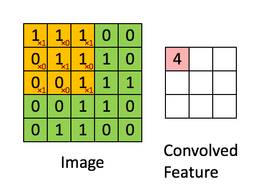
多卷积核
上面所述只有100个参数时,表明只有1个10*10的卷积核,显然,特征提取是不充分的,我们可以添加多个卷积核,比如32个卷积核,可以学习32种特征。在有多个卷积核时,如下图所示: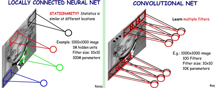
上图右,不同颜色表明不同的卷积核。每个卷积核都会将图像生成为另一幅图像。比如两个卷积核就可以将生成两幅图像,这两幅图像可以看做是一张图像的不同的通道。如下图所示,下图有个小错误,即将w1改为w0,w2改为w1即可。下文中仍以w1和w2称呼它们。
下图展示了在四个通道上的卷积操作,有两个卷积核,生成两个通道。其中需要注意的是,四个通道上每个通道对应一个卷积核,先将w2忽略,只看w1,那么在w1的某位置(i,j)处的值,是由四个通道上(i,j)处的卷积结果相加然后再取激活函数值得到的。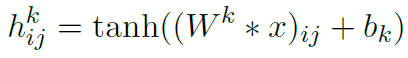
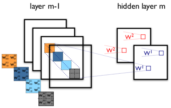
所以,在上图由4个通道卷积得到2个通道的过程中,参数的数目为4×2×2×2个,其中4表示4个通道,第一个2表示生成2个通道,最后的2×2表示卷积核大小。
Down-pooling
在通过卷积获得了特征(features)之后,下一步我们希望利用这些特征去做分类。理论上讲,人们可以用所有提取得到的特征去训练分类器,例如softmax分类器,但这样做面临计算量的挑战。例如:对于一个96X96像素的图像,假设我们已经学习得到了400个定义在8X8输入上的特征,每一个特征和图像卷积都会得到一个 (96 − 8 + 1) × (96 − 8 + 1) = 7921 维的卷积特征,由于有 400 个特征,所以每个样例 (example) 都会得到一个 7921 × 400 = 3,168,400 维的卷积特征向量。学习一个拥有超过3百万特征输入的分类器十分不便,并且容易出现过拟合 (over-fitting)。
为了解决这个问题,首先回忆一下,我们之所以决定使用卷积后的特征是因为图像具有一种“静态性”的属性,这也就意味着在一个图像区域有用的特征极有可能在另一个区域同样适用。因此,为了描述大的图像,一个很自然的想法就是对不同位置的特征进行聚合统计,例如,人们可以计算图像一个区域上的某个特定特征的平均值(或最大值)。这些概要统计特征不仅具有低得多的维度 (相比使用所有提取得到的特征),同时还会改善结果(不容易过拟合)。这种聚合的操作就叫做池化 (pooling),有时也称为平均池化或者最大池化(取决于计算池化的方法)。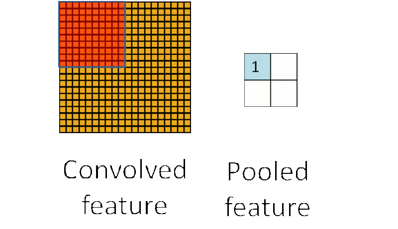
子采样有两种形式,一种是均值子采样(mean-pooling),一种是最大值子采样(max-pooling)。两种子采样看成特殊的卷积过程,如图下图所示:
(1)均值子采样的卷积核中每个权重都是0.25,卷积核在原图inputX上的滑动的步长为2。均值子采样的效果相当于把原图模糊缩减至原来的1/4。
(2)最大值子采样的卷积核中各权重值中只有一个为1,其余均为0,卷积核中为1的位置对应inputX被卷积核覆盖部分值最大的位置。卷积核在原图inputX上的滑动步长为2。最大值子采样的效果是把原图缩减至原来的1/4,并保留每个2*2区域的最强输入。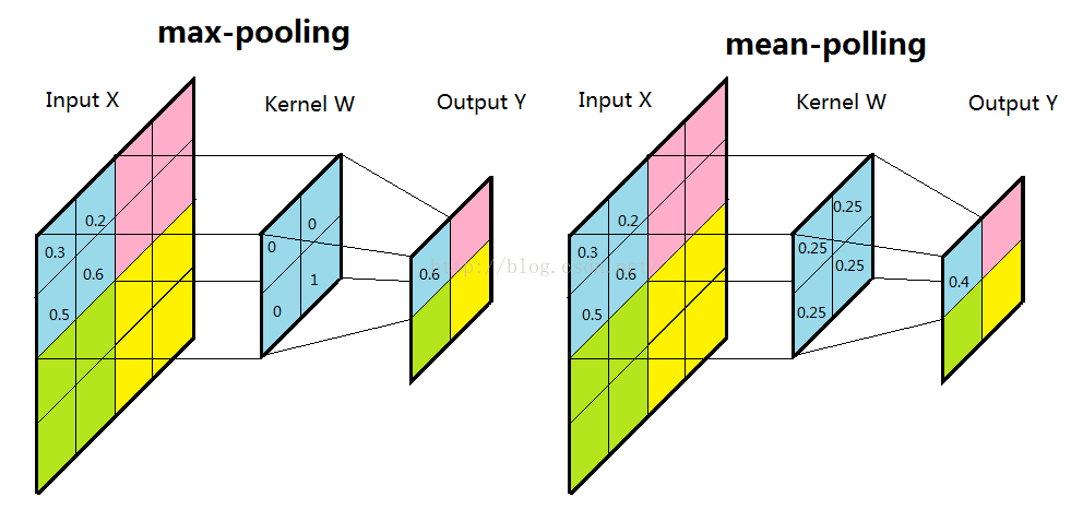
至此,卷积神经网络的基本结构和原理已经阐述完毕。
多卷积层
在实际应用中,往往使用多层卷积,然后再使用全连接层进行训练,多层卷积的目的是一层卷积学到的特征往往是局部的,层数越高,学到的特征就越全局化。
卷积神经网络的训练
本文的主要目的是介绍CNN参数在使用bp算法时该怎么训练,毕竟CNN中有卷积层和下采样层,虽然和MLP的bp算法本质上相同,但形式上还是有些区别的,很显然在完成CNN反向传播前了解bp算法是必须的。
Forward前向传播
前向过程的卷积为典型valid的卷积过程,即卷积核kernalW覆盖在输入图inputX上,对应位置求积再求和得到一个值并赋给输出图OutputY对应的位置。每次卷积核在inputX上移动一个位置,从上到下从左到右交叠覆盖一遍之后得到输出矩阵outputY(如图4.1与图4.3所示)。如果卷积核的输入图inputX为MxNx大小,卷积核为MwNw大小,那么输出图Y为(Mx-Mw+1)*(Nx-Nw+1)大小。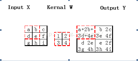
BackForward反向传播
在错误信号反向传播过程中,先按照神经网络的错误反传方式得到尾部分类器中各神经元的错误信号,然后错误信号由分类器向前面的特征抽取器传播。错误信号从子采样层的特征图(subFeatureMap)往前面卷积层的特征图(featureMap)传播要通过一次full卷积过程来完成。这里的卷积和上一节卷积的略有区别。如果卷积核kernalW的长度为MwMw的方阵,那么subFeatureMap的错误信号矩阵Q_err需要上下左右各拓展Mw-1行或列,与此同时卷积核自身旋转180度。subFeatureMap的错误信号矩阵P_err等于featureMap的误差矩阵Q_err卷积旋转180度的卷积核W_rot180。
下图错误信号矩阵Q_err中的A,它的产生是P中左上22小方块导致的,该22的小方块的对A的责任正好可以用卷积核W表示,错误信号A通过卷积核将错误信号加权传递到与错误信号量为A的神经元所相连的神经元a、b、d、e中,所以在下图中的P_err左上角的22位置错误值包含A、2A、3A、4A。同理,我们可以论证错误信号B、C、D的反向传播过程。综上所述,错误信号反向传播过程可以用下图中的卷积过程表示。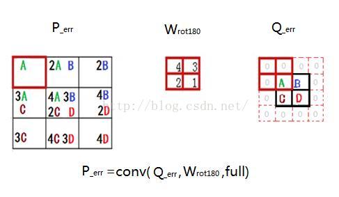
权值更新过程中的卷积
卷积神经网络中卷积层的权重更新过程本质是卷积核的更新过程。由神经网络的权重修改策略我们知道一条连接权重的更新量为该条连接的前层神经元的兴奋输出乘以后层神经元的输入错误信号,卷积核的更新也是按照这个规律来进行。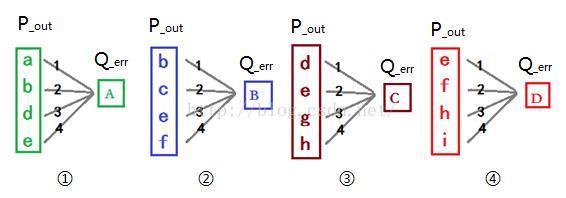
在前向卷积过程中,卷积核的每个元素(链接权重)被使用过四次,所以卷积核每个元素的产生四个更新量。把前向卷积过程当做切割小图进行多个神经网络训练过程,我们得到四个4*1的神经网络的前层兴奋输入和后层输入错误信号,如图所示。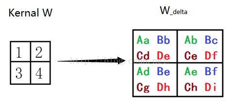
根据神经网络的权重修改策略,我们可以算出如图所示卷积核的更新量W_delta。权重更新量W_delta可由P_out和Q_err卷积得到,如图下图所示。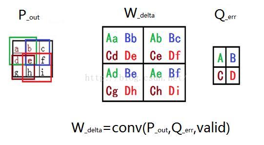
常见网络结构
ImageNet-2010网络结构
ImageNet LSVRC是一个图片分类的比赛,其训练集包括127W+张图片,验证集有5W张图片,测试集有15W张图片。本文截取2010年Alex Krizhevsky的CNN结构进行说明,该结构在2010年取得冠军,top-5错误率为15.3%。值得一提的是,在今年的ImageNet LSVRC比赛中,取得冠军的GoogNet已经达到了top-5错误率6.67%。可见,深度学习的提升空间还很巨大。
下图即为Alex的CNN结构图。需要注意的是,该模型采用了2-GPU并行结构,即第1、2、4、5卷积层都是将模型参数分为2部分进行训练的。在这里,更进一步,并行结构分为数据并行与模型并行。数据并行是指在不同的GPU上,模型结构相同,但将训练数据进行切分,分别训练得到不同的模型,然后再将模型进行融合。而模型并行则是,将若干层的模型参数进行切分,不同的GPU上使用相同的数据进行训练,得到的结果直接连接作为下一层的输入。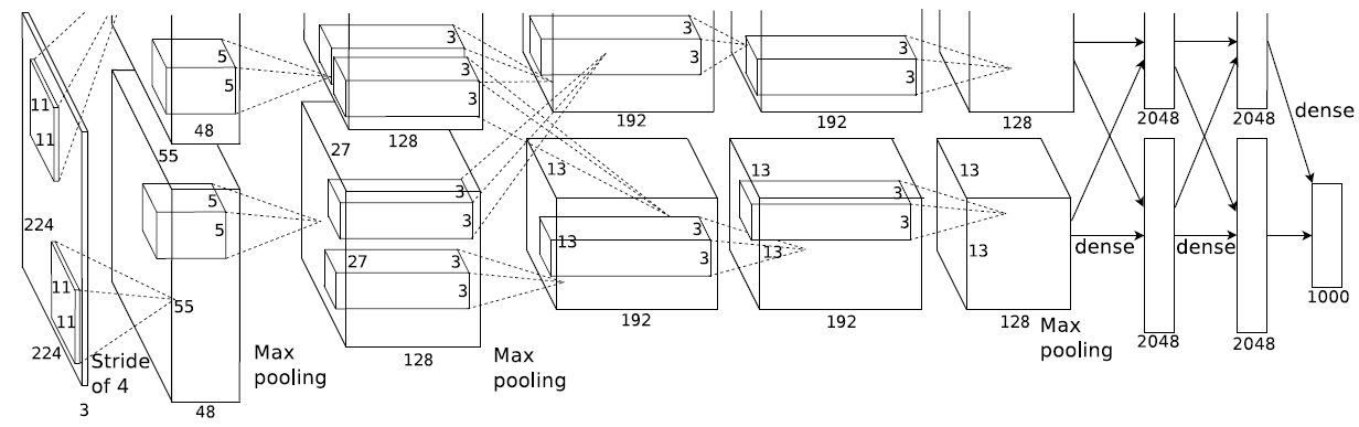
上图模型的基本参数为:
- 输入:224×224大小的图片,3通道
- 第一层卷积:11×11大小的卷积核96个,每个GPU上48个。
- 第一层max-pooling:2×2的核。
- 第二层卷积:5×5卷积核256个,每个GPU上128个。
- 第二层max-pooling:2×2的核。
- 第三层卷积:与上一层是全连接,3*3的卷积核384个。分到两个GPU上个192个。
- 第四层卷积:3×3的卷积核384个,两个GPU各192个。该层与上一层连接没有经过pooling层。
- 第五层卷积:3×3的卷积核256个,两个GPU上个128个。
- 第五层max-pooling:2×2的核。
- 第一层全连接:4096维,将第五层max-pooling的输出连接成为一个一维向量,作为该层的输入。
- 第二层全连接:4096维
- Softmax层:输出为1000,输出的每一维都是图片属于该类别的概率。
DeepID网络结构
DeepID网络结构是香港中文大学的SunYi开发出来用来学习人脸特征的卷积神经网络。每张输入的人脸被表示为160维的向量,学习到的向量经过其他模型进行分类,在人脸验证试验上得到了97.45%的正确率,更进一步的,原作者改进了CNN,又得到了99.15%的正确率。
如下图所示,该结构与ImageNet的具体参数类似,所以只解释一下不同的部分吧。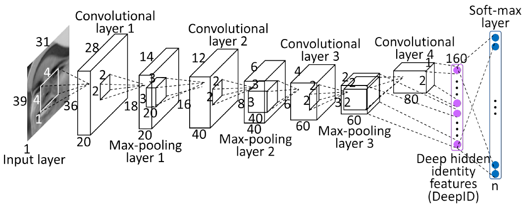
上图中的结构,在最后只有一层全连接层,然后就是softmax层了。论文中就是以该全连接层作为图像的表示。在全连接层,以第四层卷积和第三层max-pooling的输出作为全连接层的输入,这样可以学习到局部的和全局的特征。
参考资源
[1] http://deeplearning.stanford.edu/wiki/index.php/UFLDL%E6%95%99%E7%A8%8B 栀子花对Stanford深度学习研究团队的深度学习教程的翻译
[2] http://blog.csdn.net/zouxy09/article/details/14222605 csdn博主zouxy09深度学习教程系列
[3] http://deeplearning.net/tutorial/ theano实现deep learning
[4] Krizhevsky A, Sutskever I, Hinton G E. Imagenet classification with deep convolutional neural networks[C]//Advances in neural information processing systems. 2012: 1097-1105.
[5] Sun Y, Wang X, Tang X. Deep learning face representation from predicting 10,000 classes[C]//Computer Vision and Pattern Recognition (CVPR), 2014 IEEE Conference on. IEEE, 2014: 1891-1898.
[6] http://blog.csdn.net/stdcoutzyx/article/details/41596663
[7] http://blog.csdn.net/yunpiao123456/article/details/52437794
Original: Large column article read convolution neural network CNN