Using a linear least squares fit in

1, the relevant API

　　(1), the value of the most

　　　　np.max () np.min () np.ptp ( ): returns an array of the maximum / minimum / poor

　　　　np.argmax () np.argmin (): subscript returns an array of the maximum / minimum element

　　　　np.maximum () np.minimum (): the elements of the maximum / minimum elements corresponding to the same two-dimensional array to form a new array

　　(2), as specified in an array along the axial direction, call handler, and returns the value returned again organized into arrays each call.

DEF FUNC (Data):
     Pass 
# FUNC handler 
# Axis axial [0,1] 
# Array array 
np.apply_along_axis (func, axis, array)

　　(3), convolution

= C numpy.convolve (A, b, convolution type) 

A = [. 1, 2,. 3,. 4,. 5 ] the original array 
b = [. 8,. 7,. 6 ] convolution kernel array 

used as a convolution kernel b, of a process of performing convolution operation of the array as follows:
            446,586          valid convolution (valid)
         23 is 446586 59       with dimensional convolution (same)
       . 8 59 446 586 30 23 is    complete convolution (full) 
0 0   . 1 2. 4. 3 . 5   0 0
 . 6. 7. 8 
   . 6. 7. 8 
      . 6. 7. 8 
         . 6. 7. 8 
            . 6. 7. 8 
               . 6. 7. 8 
                  . 6. 7. 8

　　(4), in line with the least squares method to calculate the minimum error fitting coefficients (the only solution is not required, but required the minimum error solution)

= X np.linalg.lstsq (A, B) [0]
 # A, B is a sample value

　　(5), the arithmetic mean and a weighted average,

Arithmetic mean: 
np.mean (Array) 
or array.mean () 
Weighted average: 
np.average (closing_prices, Volumes weights =) 
Note: The arithmetic mean is a weighted average understood equally weighted.

　　(6) Other

Median: median, poor: ptp.

2, the correlation matrix

　　

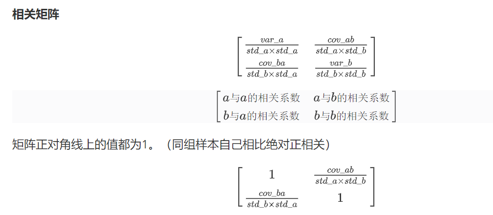
numpy.corrcoef (A, B)         # find correlation matrix 
numpy.cov (A, B)     # Covariance Matrix

3, polynomial fitting related API

The fitted values obtained from the fit coefficients and variables, whereby to obtain the sample data curve fit coordinates [X-, the Y ' ] 
np.polyval (P, X-) -> the Y '
 
polynomial derivation function, fitting coefficients according to obtaining the derivatives of the polynomial function coefficients 
np.polyder (P) -> Q 

known polynomial coefficients of the polynomial roots find Q (x-axis and the abscissa intersection) 
XS = np.roots (Q) 

two polynomial function of the difference between coefficients of the functions (the intersection of the two curves may be ascertained through the root difference function) 
Q = np.polysub (Pl, P2)

4, data smoothing

　　Smoothing processing generally comprises a noise data fitting and other operations. Intended for purposes of noise reduction features remove additional factors, intended to fit the mathematical modeling, mathematical methods can be more identifying characteristic curve.