Grid search with K-nearest neighbor in more hyperparameter

Grid search with K-nearest neighbor in more hyperparameter

---

Grid search, the Grid Search: An ultra parameter optimization means; all parameter candidates selected by looping through, try every possibility, the best performance parameter is the final result. (Why is it called grid search? There are two parameters to the model as an example, there are three possible parameters a, b parameters there are four possibilities, all possibilities listed, the table can be expressed as a 3 * 4 cycle it is like in each grid traversal, search, so called grid search)

A, knn grid search optimization hyperparametric

1. First, prepare data sets.

from sklearn import datasets
from sklearn.metrics import accuracy_score
from sklearn.model_selection import train_test_split
from sklearn.neighbors import KNeighborsClassifier

digits = datasets.load_digits()
x = digits.data
y = digits.target

x_train, x_test, y_train, y_test = train_test_split(x, y, test_size=0.2)

2. Create a Web search parameters:

param_grid = [
    {
        'weights':['uniform'],
        'n_neighbor':[i for i in range(1, 11)]
    },
    {
        'weights':['distance'],
         'n_neighbor':[i for i in range(1, 11)],
        'p':[i for i in range(1, 6)]
    }
]

1. Knn the beginning of the super-reference search:

from sklearn.neighbors import KNeighborsClassifier
from sklearn.model_selection import GridSearchCV

knn_clf = KNeighborsClassifier()
grid_search = GridSearchCV(knn_clf, param_grid)

%%time
grid_search.fit(x_train, y_train)

Output:

Wall time: 2min 20s

GridSearchCV(cv='warn', error_score='raise-deprecating',
       estimator=KNeighborsClassifier(algorithm='auto', leaf_size=30, metric='minkowski',
           metric_params=None, n_jobs=None, n_neighbors=5, p=2,
           weights='uniform'),
       fit_params=None, iid='warn', n_jobs=None,
       param_grid=[{'weights': ['uniform'], 'n_neighbors': [1, 2, 3, 4, 5, 6, 7, 8, 9, 10]}, {'weights': ['distance'], 'n_neighbors': [1, 2, 3, 4, 5, 6, 7, 8, 9, 10], 'p': [1, 2, 3, 4, 5]}],
       pre_dispatch='2*n_jobs', refit=True, return_train_score='warn',
       scoring=None, verbose=0)

grid_search.best_estimator_
grid_search.best_score_
grid_search.best_params_

knn_clf = grid_search.best_estimator_
knn_clf.predict(x_test)
knn_clf.score(x_test, y_test)

In fact, this kind of hyper-parameters GridSearch there metric_params, metrics and so on. There are also some help us better understand grid search parameters, such as n_jobs indicates how many nuclear computer use. If all indication -1 core. For example, in the search process can be displayed in a number of log information, verbose, the larger the value of the output value of the detail, and generally 2 suffice.

%%time
grid_search = GridSearchCV(knn_clf, param_grid, n_jobs=-1, verbose=2)
grid_search.fit(x_train, y_train)

Output:

Fitting 3 folds for each of 60 candidates, totalling 180 fits

[Parallel(n_jobs=-1)]: Done  29 tasks      | elapsed:    9.5s
[Parallel(n_jobs=-1)]: Done 150 tasks      | elapsed:   28.7s

Wall time: 35.5 s

[Parallel(n_jobs=-1)]: Done 180 out of 180 | elapsed:   35.4s finished

Second, more defined distance

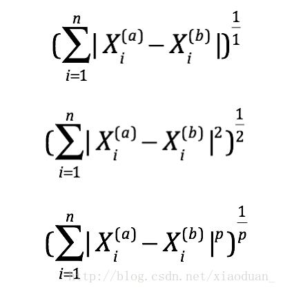
If the distance in knn this parameter is used by default Minkowski distance, wherein if p is 1, is a Manhattan distance, and p is 2, is the Euclidean distance. In addition to these there are some distance definition:

• Manhattan distance

  For example, on a plane, Manhattan distance coordinate (x1, y1) and the coordinates of the point i (x2, y2) is a point j:

  d(i,j)=|X1-X2|+|Y1-Y2|.

  

• Euclidean distance

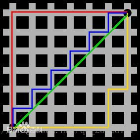
• Minkowski distance

  Manhattan can be seen as the promotion of distance and Euclidean distance.

In mathematics, the distance is a strict definition, need to meet three properties: non-negative, symmetrical triangle inequality.

1, cosine similarity vector space

Cosine similarity, also known as the cosine similarity is calculated by two vector angle cosine to evaluate their similarity values.

The cosine value between two vectors by using the Euclidean dot product equation is obtained:

​ 余弦距离，就是用1减去这个获得的余弦相似度。余弦距离不满足三角不等式，严格意义上不算是距离。

2、调整余弦相似度

​ 修正cosine相似度的目的是解决cosine相似度仅考虑向量维度方向上的相似而没考虑到各个维度的量纲的差异性，所以在计算相似度的时候，做了每个维度减去均值的修正操作。

​ 比如现在有两个点：（1,2）和（4,5），使用余弦相似度得到的结果是0.98。余弦相似度对数值的不敏感导致了结果的误差，需要修正这种不合理性就出现了调整余弦相似度，即所有维度上的数值都减去一个均值。那么调整后为（-2，-1）和（1,2），再用余弦相似度计算，得到-0.8。

3、皮尔森相关系数

​ 也称皮尔森积矩相关系数(Pearson product-moment correlation coefficient) ，是一种线性相关系数。皮尔森相关系数是用来反映两个变量线性相关程度的统计量。

​ 两个变量之间的皮尔逊相关系数定义为两个变量之间的协方差和标准差的商：

​ 对比协方差公式：皮尔逊相关系数由两部分组成，分子是协方差公式，分母是两个变量的方差乘积。协方差公式有一些缺陷，虽然能反映两个随机变量的相关程度，但其数值上受量纲的影响很大，不能简单地从协方差的数值大小给出变量相关程度的判断。所以，皮尔森相关系数用方差乘积来消除量纲的影响。

4、杰卡德相似系数

• 杰卡德相似系数

  两个集合A和B交集元素的个数在A、B并集中所占的比例，称为这两个集合的杰卡德系数。

  

• 杰卡德距离

  杰卡德距离用两个两个集合中不同元素占所有元素的比例来衡量两个集合的区分度。