KNN algorithm works:
KNN (k-nearest neighbor) is a simple and classic machine learning classification algorithm (usually a Euclidean distance) to classify the samples by measuring "data to be classified" distance "category known sample" of.
This point was some convoluted, and to break down some:
(1) classification are supervised (supervised) problem, that is to say a certain number of sample categories are known.
(2) Now that we have a number of the sorted samples, then the next natural work should be known samples by training a classifier (by adjusting the parameters of the classifier, the classifier to correctly classify training samples), the classifier training is good for the future classification of unknown samples (or class prediction).
Looked like such a thing, the key issue is to train the classifier.
But for the KNN classifier, things are not like this. In fact, KNN is not so complicated. KNN parameters because there is nothing to adjust, in other words, KNN actually do not need training!
As the most simple and best appreciated classifier, the KNN just assume that the data are distributed in European feature space (the coordinates in distinguishing spatial characteristic value of different samples), then we know exactly the position and all the data in this space, and wherein a portion of the data category. So now we have to determine how the remaining categories of data that it?
In order to classify proceed, in fact, here we assume that: space closer distances greater the likelihood of a point belonging to the class.
With this "axiom", that things would be much easier. We just need to calculate the distance to be classified in each category of data to all known data just fine. Figure:

There are two known classes squares and triangles, if the center of the circular We do not know in the end is triangular or square. According to the above said, we can now eight children calculate its distance to all other points. For simplicity here, we find that it is from the visual look next to the triangle Recently Go ahead, then we put it classified as a kind of triangle.
Note that here we have an unknown point and the nearest point that a classified as a class. Such a classifier, precisely called nearest neighbor classifier (nearest-neighbor, NN). This is a special case KNN, is the case of K = 1.
So K-nearest neighbor, by definition, is unknown to a reference point from its nearest first k classes have been the point, look at the k points inside, up to the point belongs to which category, it considers that an unknown point which category. FIG above or to the unknown point as the center circle, the circle drawn in solid line, corresponding to k = 3, is selected from the first three nearest point from which the two triangle, a square, Therefore, unknown point attributed to a class of a triangle. However, when considering the dashed line, i.e. k = 5, we found three squares, two triangles, so this time the unknown point normalized to the square of a class.
So we can see a different number of nearest neighbors often lead to different classification results, in general, we have to determine the value of k in the practical application of the actual situation and experience.
The principle of self-reference section Bowen: https://blog.csdn.net/weixin_41988628/article/details/80369850
KNN classifier to classify the use of a simple two-dimensional example
Create a set of two-dimensional point code section as follows:
By way of randomly generated, creating two different two-dimensional point set class1 and Class2, each set has two points, respectively, and the normal distribution around the ring, the normal range of main parameters by adjusting tags achieve larger the parameter, the greater the range of the data points, even more dispersed.
Range distribution around the ring, the radius r of the outer ring determines the degree of concentration data set, when the larger r, the greater the range of the data, the more dispersion
# -*- coding: utf-8 -*-
#生成点的过程
from numpy.random import randn
import pickle
from pylab import *

# create sample data of 2D points
# 打印两百个点
n = 200
# two normal distributions
# 两百个二维的点并通过*0.6限制他们的范围
class_1 = 0.8 * randn(n,2)
class_2 = 1.0 * randn(n,2) + array([5,1])
# 给他们分标签
labels = hstack((ones(n),-ones(n)))
# save with Pickle
#with open('points_normal.pkl', 'w') as f:
# 把他们存进
with open('points_normal_test.pkl', 'wb') as f:
    pickle.dump(class_1,f)
    pickle.dump(class_2,f)
    pickle.dump(labels,f)
# normal distribution and ring around it
print ("save OK!")
# 环状的数据
class_1 = 0.3 * randn(n,2)
r = 0.5 * randn(n,1) + 5
angle = 2*pi * randn(n,1)
class_2 = hstack((r*cos(angle),r*sin(angle)))
labels = hstack((ones(n),-ones(n)))
# save with Pickle
#with open('points_ring.pkl', 'w') as f:
with open('points_ring_test.pkl', 'wb') as f:
    pickle.dump(class_1,f)
    pickle.dump(class_2,f)
    pickle.dump(labels,f)

print ("save OK!")
KNN classifier using the above set of points randomly generated class code are the following:
Visualization is classified all test data points, and to show how the classifier to separate two different classes, the need to create a secondary function classify (x, y, model = model), to obtain the x and y coordinates of a two-dimensional array and sorter and one predicted class returns array of tags array. Is then passed to the real function classify plot_2D_boundary drawing function as a parameter.
This requires a mapping function classifiers, and () function with a grid on predicted meshgrid now, the accuracy of the grid is 0.1, a collection every 0.1 point. Contour classifier may display position of the boundary, the boundary is zero default contours. For each category, with the correct class classification * draw, with O draw incorrect classification point
# -*- coding: utf-8 -*-
import pickle
from pylab import *
from PCV.classifiers import knn
from PCV.tools import imtools

pklist=['points_normal.pkl','points_ring.pkl']

figure()

# load 2D points using Pickle
# 枚举前面的两个元素
for i, pklfile in enumerate(pklist):
    with open(pklfile, 'rb') as f:
        class_1 = pickle.load(f)
        class_2 = pickle.load(f)
        labels = pickle.load(f)
    # load test data using Pickle
    with open(pklfile[:-4]+'_test.pkl', 'rb') as f:
        class_1 = pickle.load(f)
        class_2 = pickle.load(f)
        labels = pickle.load(f)

#knn分类器
    model = knn.KnnClassifier(labels,vstack((class_1,class_2)))
    # test on the first point
    print (model.classify(class_1[0]))

    #define function for plotting
    def classify(x,y,model=model):
        return array([model.classify([xx,yy]) for (xx,yy) in zip(x,y)])

    # lot the classification boundary
    subplot(1,2,i+1)
    # 画分界线
    imtools.plot_2D_boundary([-6,6,-6,6],[class_1,class_2],classify,[1,-1])
    titlename=pklfile[:-4]
    title(titlename)
show()
Using the above code is run out of the results is shown below, good results were classified datasets, but no dense case misclassification

Below normal range of adjustment of some denser, the normal set point code is modified as follows the range form
class_1 = 0.8 * randn(n,2)
class_2 = 1.0 * randn(n,2) + array([5,1])
Classification results have found cases of misclassification, misclassification of points indicated by circles.
Implement (dense) sift dense feature image
code show as below:
# -*- coding: utf-8 -*-
from PCV.localdescriptors import sift, dsift
from pylab import  *
from PIL import Image

dsift.process_image_dsift('gesture/wenwen.jpg','wenwen.dsift',90,40,True)
#读取dsif文件
l,d = sift.read_features_from_file('wenwen.dsift')
im = array(Image.open('gesture/wenwen.jpg'))
sift.plot_features(im,l,True)
title('dense SIFT')
show()
FIG operation results as follows:

The code dsift.process_image_dsift ( 'gesture / wenwen.jpg', 'wenwen.dsift', 90,40, True) indicates the size of the circles 90, 40 denotes a step, when the size of the same holding ring, the step becomes Great results FIG 80 is as follows:

These results indicate that in the case where the same size of the circle, with the step increases the greater the distance between the center point of the circle
Image Classification - implement gesture recognition
Gesture code visualization with the image descriptors are as follows:
With dense SIFT descriptor to represent these test above gesture images, and records the test data set into the database. The image creation code would specify a signature file suffix .dsift
# -*- coding: utf-8 -*-
import os
from PCV.localdescriptors import sift, dsift
from pylab import  *
from PIL import Image

imlist=['gesture/wen/C-uniform02.jpg','gesture/wen/B-uniform01.jpg',
        'gesture/wen/A-uniform01.jpg','gesture/wen/Five-uniform01.jpg',
        'gesture/wen/Point-uniform01.jpg','gesture/wen/V-uniform01.jpg']

figure()
for i, im in enumerate(imlist):
    print (im)
    dsift.process_image_dsift(im,im[:-3]+'dsift',40,20,True)
    l,d = sift.read_features_from_file(im[:-3]+'dsift')
    dirpath, filename=os.path.split(im)
    im = array(Image.open(im))
    #显示手势含义title
    titlename=filename[:-14]
    subplot(2,3,i+1)
    sift.plot_features(im,l,True)
    title(titlename)
show()
Operating results are as follows:

Recognized by the gesture data training code is as follows:
After the operation results will be used to display the correct rate of testing for a given set how many images are correctly classified, but it does not tell us what gestures are difficult to classify, or which mistakes. At this time, we can show case misclassified by confusion matrix. Is a confusion matrix can show how many of each type of sample is divided in each category of the matrix, it can display an error distribution, as well as which classes are often each other "confused" in
# -*- coding: utf-8 -*-
from PCV.localdescriptors import dsift
import os
from PCV.localdescriptors import sift
from pylab import *
from PCV.classifiers import knn

def get_imagelist(path):
    """    Returns a list of filenames for
        all jpg images in a directory. """
#获取图片的路径
    return [os.path.join(path,f) for f in os.listdir(path) if f.endswith('.jpg')]

def read_gesture_features_labels(path):
    # create list of all files ending in .dsift
    featlist = [os.path.join(path,f) for f in os.listdir(path) if f.endswith('.dsift')]
    # read the features
    features = []
    for featfile in featlist:
        l,d = sift.read_features_from_file(featfile)
        features.append(d.flatten())
    features = array(features)
    # create labels
    labels = [featfile.split('/')[-1][0] for featfile in featlist]
    return features,array(labels)

def print_confusion(res,labels,classnames):
    n = len(classnames)
    # confusion matrix
    class_ind = dict([(classnames[i],i) for i in range(n)])
    confuse = zeros((n,n))
    for i in range(len(test_labels)):
        #是正确的类别就加一
        confuse[class_ind[res[i]],class_ind[test_labels[i]]] += 1
    print ('Confusion matrix for')
    print (classnames)
    print (confuse)

filelist_train = get_imagelist('gesture/train')
filelist_test = get_imagelist('gesture/test')
imlist=filelist_train+filelist_test

# process images at fixed size (50,50)
for filename in imlist:
    featfile = filename[:-3]+'dsift'
    dsift.process_image_dsift(filename,featfile,10,5,resize=(50,50))

features,labels = read_gesture_features_labels('gesture/train/')
test_features,test_labels = read_gesture_features_labels('gesture/test/')
classnames = unique(labels)

# test kNN
k = 1
knn_classifier = knn.KnnClassifier(labels,features)
res = array([knn_classifier.classify(test_features[i],k) for i in
range(len(test_labels))])
# accuracy
acc = sum(1.0*(res==test_labels)) / len(test_labels)
print ('Accuracy:', acc)

print_confusion(res,test_labels,classnames)
# 结果竖着看,其他数值表示错判的类别
Operating results are as follows:
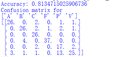
The results show that the correct classification rate of 81.3%
混淆矩阵竖着看,比如A列,分类正确的有26,将A分错成V有三个
A、B、C、F、V的分类结果都比较好,错误率较低
而P类错分成V的概率很高