
Author: Yu Fan
background
The development of artificial intelligence (AI) has introduced a new paradigm to scientific discovery. Today, AI has begun to improve, accelerate, and enable our understanding of natural phenomena across a wide range of spatial and temporal scales, thereby promoting the development of natural science and giving birth to the new research field of AI4Science. Recently, a review paper "Artificial Intelligence for Science in Quantum, Atomistic, and Continuum Systems" jointly written by more than 60 authors provides an in-depth technical summary in the subfields of subatomic, atomic, and continuum systems. Here we extract the technical backbone of this review and focus on how to construct an equivariant model under symmetry transformation.
1 Introduction
In 1929, quantum physicist Paul Dirac noted: "The fundamental physical laws required for the mathematical theory of most of physics and all of chemistry are already completely known to us, and the difficulty lies in the fact that the precise application of these laws leads to complex This is true from the Schrödinger equation in quantum physics to the Navier-Stokes equation in fluid mechanics. Deep learning can speed up the solution of these equations. Using the results of traditional simulation methods as training data, once trained, these models can make predictions much faster than traditional simulation.
In other fields, such as biology, the underlying biophysical processes may not be fully understood and may ultimately not be described by mathematical equations. In these cases, deep learning models can be trained using experimentally generated data, such as protein prediction models AlphaFold, RoseTTAFold, ESMFold, and other 3D structures obtained through experiments, so that the accuracy of computationally predicted protein 3D structures can be comparable to experimental results. .
1.1 Scientific fields
The scientific areas of interest in this article are organized as an overview in the figure below, according to the spatial and temporal scales of the physical system being modeled.
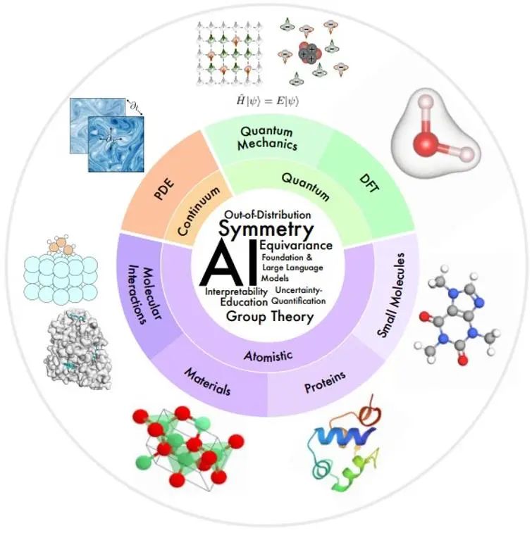
Small scale: Quantum mechanics uses the wave function to study physical phenomena at the smallest scale. The Schrödinger equation it obeys describes the complete dynamic process of the quantum system, but it brings exponential complexity. Density functional theory (DFT) and ab initio quantum chemistry methods are first-principles methods widely used in practice to calculate the electronic structure and physical properties of molecules and materials, and can further deduce the electronic and mechanical properties of molecules and solids. , optical, magnetic and catalytic properties. However, these methods are still computationally expensive, limiting their use to small systems (~1000 atoms). The AI model can help improve speed and accuracy.
Mesoscale: Small molecules, typically tens to hundreds of atoms in size, play important regulatory and signaling roles in many chemical and biological processes. Proteins are large molecules composed of one or more amino acid chains. Amino acid sequence determines protein structure, which in turn determines their function. Materials science research studies the relationship between processing, structure, properties and materials. Molecular interactions study how many physical and biological functions are performed through molecular interactions, such as ligand-receptor and molecule-material interactions. In these fields, AI has made many progress in molecular characterization and generation, molecular dynamics, protein structure prediction and design, material property prediction and structure generation.
Large scale: Continuum mechanics uses partial differential equations to model physical processes that evolve in time and space at the macroscopic level, including fluid flow, heat transfer, electromagnetic waves, etc. AI methods provide some solutions to problems such as improving computational efficiency, generalization, and multi-resolution analysis.
1.2 AI technology field
A common set of technical challenges exists across multiple areas of scientific AI.
**Symmetry:**Symmetry is a very strong inductive paranoia, so a key challenge for AI4Science is how to effectively integrate symmetry in AI models.
**Interpretability:**Interpretability is crucial in AI4Science to understand the laws of the physical world.
**Out-of-distribution (OOD) generalization and causality: **To avoid generating training data for each different setting, causal factors that enable OOD generalization need to be identified.
**Basic models and large language models:**Basic models in natural language processing tasks are pre-trained under self-supervised or generalizable supervision to perform various downstream tasks in a few-shot or zero-shot manner. The article provides perspective on how this paradigm can accelerate AI4Science discoveries.
**Uncertainty Quantification (UQ): **Studies how to ensure robust decision making under data and model uncertainty.
**Education:** To facilitate learning and education, this article provides a categorized list of resources that the author finds useful, and provides perspectives on how the community can better promote the integration of AI with science and education.
**2. ** Symmetry, equivariance, and their theories
In many scientific problems, the object of interest is usually located in 3D space, and any mathematical representation of the object relies on a reference coordinate system, making such a representation relative to the coordinate system. However, coordinate systems do not exist in nature, so a coordinate system-independent representation is needed. Therefore, one of the key challenges of AI4Science is how to achieve invariance or equivariance under coordinate system transformation.
2.1 Overview
Symmetry refers to the fact that the properties of a physical phenomenon remain unchanged under certain transformations, such as coordinate transformations. If certain symmetries exist in the system, the prediction target is naturally invariant or equivariant under the corresponding symmetry transformation. For example, when predicting the energy of a 3D molecule, the predicted value remains unchanged when the 3D molecule is translated or rotated. An alternative strategy to achieve symmetry-aware learning is to use data augmentation in supervised learning, specifically applying random symmetry transformations to the input data and labels to force the model to output approximately equivariant predictions. But this has many disadvantages:
1) Taking into account the additional degrees of freedom in selecting the coordinate system, the model requires greater capacity to represent patterns that are originally simple in a fixed coordinate system;
2) Many symmetry transformations, such as translation, can produce an infinite number of equivariant samples, making it difficult for limited data enhancement to fully reflect the symmetry in the data;
3) In some cases, it is necessary to build a very deep model to achieve good prediction results. If each layer of the model cannot maintain equivariance, it will be difficult to predict the overall output of equivariance;
4) In scientific problems such as molecular modeling, it is crucial to provide a prediction that is robust under symmetry transformations so that machine learning can be used in a trustworthy manner.
Due to the many shortcomings of data augmentation, more and more research focuses on designing machine learning models that meet symmetry requirements. Under the symmetry adaptation architecture, the model can focus on the learning target prediction task without data enhancement.
2.2 Equivariability under discrete symmetry transformation
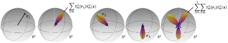
In this section, the author provides an example of maintaining equivariance under discrete symmetry transformations in an AI model. This example problem simulates the mapping of a scalar flow field in a 2D plane from one moment to the next. When the input flow field rotates 90, 180, and 270 degrees, the output flow field will also rotate accordingly. Its mathematical expression is as follows:
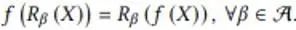
where f represents the flow field mapping function and R represents the discrete rotation transformation. Cohen et al. proposed equivariant group convolutional neural networks (G-CNNs) to solve this problem. Its simplest basic component is ascending dimension convolution:
1) First rotate the convolution kernel at all angles in the symmetric transformation, and use the rotated convolution kernel to perform corresponding convolution operations on the input to obtain multiple feature layers, and stack these feature layers in the newly generated rotation dimension α Together; 2) Pooling is performed in this rotation dimension α, so that the resulting output will produce a corresponding rotation when the input X is rotated.
Due to the existence of the pooling operation, although the equivariant rows are maintained, these features cannot carry direction information. Usually G-CNNs adopt the structure as shown in the following figure:
First, a rotational convolution kernel is used to increase the dimension of the input, then a multi-layer group convolution layer is used to make each layer of features meet the requirements of rotational equivariance while maintaining the rotational dimension, and finally a pooling layer is used to eliminate the rotational dimension. This allows the intermediate feature layer to better detect patterns in relative positions and orientations of features. The meaning of the equivariance of the intermediate feature layer is that the feature layer rotates accordingly under the rotation transformation, and the order in the rotation dimension also rotates; and the rotation and rotation design of the convolution kernel in the group convolution layer used also makes the output The feature layer can maintain this equivariance characteristic.
2.3-2.5 Construction of equivariant model of 3D continuous transformation
In many scientific problems, we focus on continuous rotation and translation symmetries in 3D space. For example, when the structure of chemical molecules rotates and translates, the vector composed of predicted molecular attributes will undergo corresponding transformations. These continuous rotation transformations R and translation transformations t constitute the elements in the SE(3) group, and these transformations can be expressed as transformation matrices in vector space. The transformation matrices in different vector spaces may be different, but these vector spaces can be decomposed into independent sub-vector spaces. There are the same transformation rules in each subspace, that is, the vector obtained by applying all the transformation elements in the group to the vector of the subspace is still in the subspace. Therefore, the transformation elements in the group can be irreducible in the subspace. Transformation matrix representation. For example, scalar quantities such as total energy and energy gap remain unchanged under the action of SE(3) group elements, and their transformation matrix is expressed as D^0(R)=1; the force field and other 3D vectors of SE(3) group elements Corresponding rotation occurs under the action, and its transformation matrix is expressed as D^1(R)=R; in a higher-dimensional vector space, D^l(R) is a 2l+1-dimensional square matrix. These transformation matrices D^l(R) are called the l-order Wigner-D matrix corresponding to the rotation R, and the corresponding sub-vector space becomes the l-order irreducible invariant subspace of the SE(3) group, and the vector in it is called l Order equivariant vector. Under translation transformation, these vectors always remain unchanged, because the properties we care about are only related to relative positions.
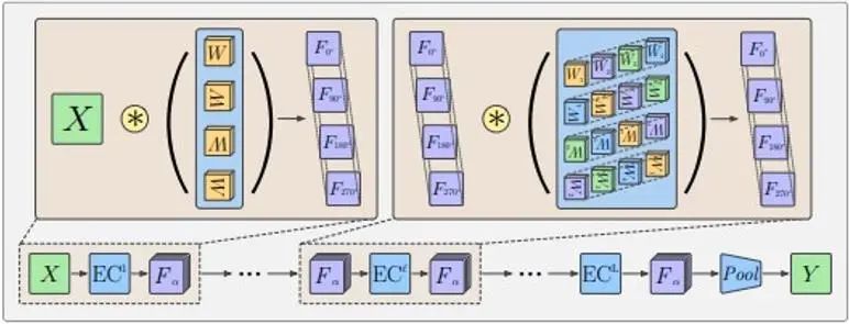
The usual way to map 3D geometric information to features in the invariant subspace of the SE(3) group is to use spherical harmonic function mapping. The spherical harmonic function Y^l maps a 3-dimensional vector into a 2l+1-dimensional vector, which represents the coefficient when the input vector is decomposed into 2l+1 basic spherical harmonic functions. As shown in the figure below, since only a limited number of bases are used, the delta function on the sphere represented by the three-dimensional vector will be broadened to a certain extent.
Spherical harmonics have the following equivariant properties:
Among them, D is the l-order Wigner-D matrix mentioned earlier. Therefore, a space function is decomposed into a combination of equivariant vectors of different orders under rotation transformation.
Assuming that in a graph neural network with atomic coordinates as nodes, the node feature h is an equivariant vector of order l_1, then the following graph information transfer and update can ensure that the updated h also maintains equivariance:
The key step in this is the tensor product operation (TP) during information transfer. Among them, vec means vectorizing the matrix, and the coefficient C is a matrix with 2l_3+1 rows (2l_1+1) (2l_2+1) columns.
The node feature h is a vector in the irreducible invariant subspace of order l_1. The spherical harmonic function Y of the edge direction r_ij is a vector in the irreducible invariant subspace of order l_2. The vector obtained by the direct product of these two vectors The space is reducible, and the coefficient C is the conversion relationship from this reducible space to an irreducible invariant subspace of order l_3. For example, the direct product space of two 3-dimensional vectors is as follows:
The rotation transformation matrix of the direct product space can be converted into the three-block diagonal matrix in the middle of the figure above, which means that this space can be decomposed into three irreducible invariant subspaces with dimensions of 1, 3, and 5, that is, 3⨂ Decomposition of the vector space of 3=1⊕3⊕5. The coefficient C is the transformation matrix from this nine-dimensional space to these 1-dimensional, 3-dimensional, and 5-dimensional spaces respectively. In the above formula, l_1, l_2, and l_3 all take only one value and are equivariant features of fixed order. The features in the actual network can be a combination of these different order features.
2.6-2.7 In the previous examples, the group theory theory and the properties of spherical harmonic functions were used. The basic knowledge of group theory and spherical harmonic functions are introduced in detail in these two chapters of the article.
2.8 The steerable kernel constitutes a general form of equivariant network
The previous equivariant network layers under discrete and continuous transformations can be described in the form of a unified variable convolution (steerable CNN):
Among them, x and y are spatial coordinates, f_in(y) represents the input feature vector at coordinate y, f_out(x) represents the output feature vector at coordinate x, and K is the transformation from the input feature space to the output feature space. The convolution operation ensures translational equivariance. In order to ensure equivariance under other spatial affine transformations, the convolution kernel K also needs to satisfy the following symmetry constraints:
Among them, g is the transformation in the space transformation group, and ρ_in and ρ_out represent the representation of the transformation in the input and output feature spaces (i.e., the transformation matrix) respectively.
At this point, the article's theoretical explanation of symmetry and equivariance has basically come to an end, followed by a separate overview of the multiple fields listed in Chapter 1.
references
[1] Ren P, Rao C, Liu Y, et al. PhyCRNet: Physics-informed convolutional-recurrent network for solving spatiotemporal PDEs[J]. Computer Methods in Applied Mechanics and Engineering, 2022, 389: 114399.
[2]https://www.sciencedirect.com/science/article/abs/pii/S0045782521006514?via%3Dihub
【1】 Xuan Zhang, Limei Wang, Jacob Helwig, et al. 2023. Artificial Intelligence for Science in Quantum, Atomistic, and Continuum Systems. arXiv: https://arxiv.org/abs/2307.08423
【2】 Taco Cohen and Max Welling. 2016. Group Equivariant Convolutional Networks. In International Conference on Machine Learning. PMLR, 48:2990–2999.
【3】 Nathaniel Thomas, Tess Smidt, Steven Kearnes, et al. 2018. Tensor field networks: Rotation-and translation-equivariant neural networks for 3d point clouds. arXiv: https://arxiv.org/abs/1802.08219
Maurice Weiler, Mario Geiger, Max Welling, et al. 2018. 3D Steerable CNNs: Learning Rotationally Equivariant Features in Volumetric Data. In Advances in Neural Information Processing Systems
A programmer born in the 1990s developed a video porting software and made over 7 million in less than a year. The ending was very punishing! Google confirmed layoffs, involving the "35-year-old curse" of Chinese coders in the Flutter, Dart and Python teams . Daily | Microsoft is running against Chrome; a lucky toy for impotent middle-aged people; the mysterious AI capability is too strong and is suspected of GPT-4.5; Tongyi Qianwen open source 8 models Arc Browser for Windows 1.0 in 3 months officially GA Windows 10 market share reaches 70%, Windows 11 GitHub continues to decline. GitHub releases AI native development tool GitHub Copilot Workspace JAVA is the only strong type query that can handle OLTP+OLAP. This is the best ORM. We meet each other too late.