Generative large language models (LLM) can generate highly fluent responses to various user prompts. However, large models tend to hallucinate or make non-factual statements, which can damage user trust.
The long, detailed output of a large language model may look convincing, but there's a good chance that these outputs are fiction. Does this mean we can’t trust chatbots and have to manually check the output for facts every time? There are ways to make chatbots less likely to tell lies with the right safeguards in place.
One of the simplest methods is to adjust the temperature to a large value, such as 0.7, and then use the same question for multiple conversations. The resulting output should only change the structure of the sentence, and the difference between the outputs should be semantic rather than factual.

This simple idea allows the introduction of a new sample-based hallucination detection mechanism. If the LLM's outputs for the same cue are conflicting, they are likely to be hallucinations. If they are correlated, it means the information is true. For this type of evaluation, we only need the textual output of llm. This is called black box evaluation.
cosine distance
Cosine distance is a measure of similarity between two vectors and is commonly used in fields such as text similarity, recommendation systems, and machine learning. We can compute the pairwise cosine similarity between corresponding pairs of embedded sentences. The function below takes as input the initially generated sentence output and a list of 3 sample outputs, sampled_passages.
The all-MiniLM-L6-v2 lightweight model is used here . Embedding a sentence turns it into its vector representation.
 output = "Evelyn Hartwell is a Canadian dancer, actor, and choreographer."
 output_embeddings= model.encode(output)

 array([ 6.09108340e-03, -8.73148292e-02, -5.30637987e-02, -4.41815751e-03,
  1.45469820e-02, 4.20340300e-02, 1.99541822e-02, -7.29453489e-02,
 …
  -4.08893749e-02, -5.41420840e-02, 2.05906332e-02, 9.94611382e-02,
  -2.24501686e-03, 2.29083393e-02, 7.80007839e-02, -9.53456461e-02],
  dtype=float32)
An embedding is generated for each output of the LLM, and the cos similarity is calculated using the pairwise_cos_sim function in sentence_transformers. The original response is compared to each new sample response and then averaged.
 from sentence_transformers.util import pairwise_cos_sim
 from sentence_transformers import SentenceTransformer

 def get_cos_sim(output,sampled_passages):
     model = SentenceTransformer('all-MiniLM-L6-v2')
     sentence_embeddings = model.encode(output).reshape(1, -1)
     sample1_embeddings = model.encode(sampled_passages[0]).reshape(1, -1)
     sample2_embeddings = model.encode(sampled_passages[1]).reshape(1, -1)
     sample3_embeddings = model.encode(sampled_passages[2]).reshape(1, -1)
     cos_sim_with_sample1 = pairwise_cos_sim(
     sentence_embeddings, sample1_embeddings
     )
     cos_sim_with_sample2  = pairwise_cos_sim(
     sentence_embeddings, sample2_embeddings
     )
     cos_sim_with_sample3  = pairwise_cos_sim(
     sentence_embeddings, sample3_embeddings
     )
     cos_sim_mean = (cos_sim_with_sample1 + cos_sim_with_sample2 + cos_sim_with_sample3) / 3
     cos_sim_mean = cos_sim_mean.item()
     return round(cos_sim_mean,2)
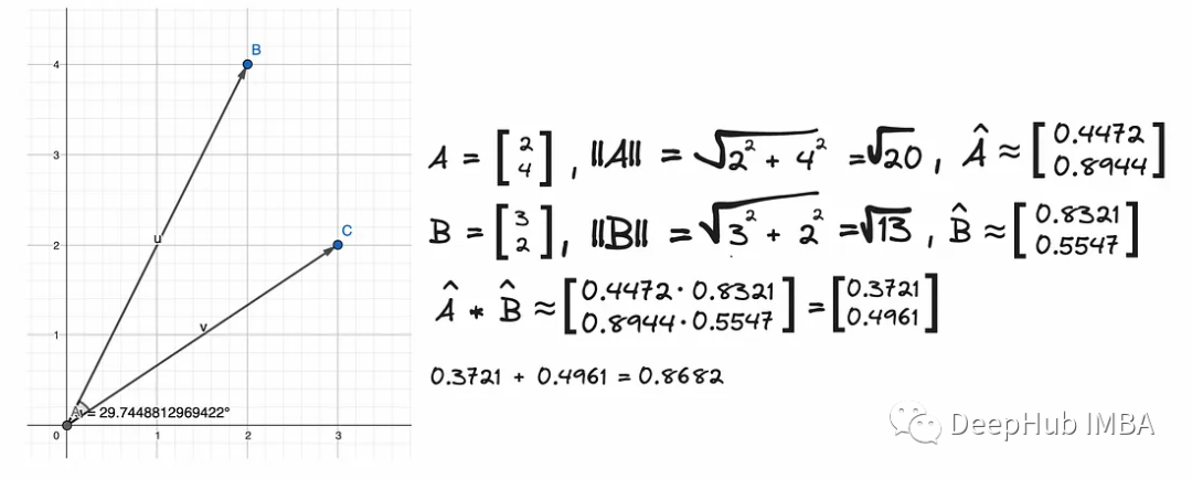
You can see from the image above that the angle between the vectors is approximately 30⁰, so they are close to each other. Cosine is approximately 0.87. The closer the cosine function is to 1, the closer the two vectors are.
cos_sim_score = get_cos_sim(output, [sample1,sample2,sample3])
The average value of embedded cos_sim_score is 0.52.
To understand how to interpret this number, let's compare it to the cosine similarity score of some valid outputs

The cosine similarity of this output is 0.93. So the first output is most likely an illusion of LLM.
BERTScore
BERTScore is based on the idea of pairwise cosine similarity.
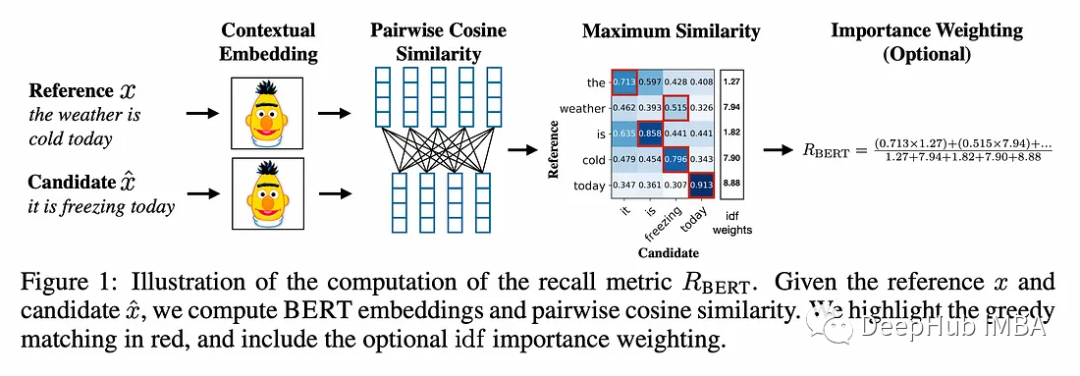
The tokenizer used to compute contextual embeddings is RobertaTokenizer. Contextual embeddings differ from static embeddings in that they take into account the context surrounding the word.
 def get_bertscore(output, sampled_passages):
     # spacy sentence tokenization
     sentences = [sent.text.strip() for sent in nlp(output).sents]
     selfcheck_bertscore = SelfCheckBERTScore(rescale_with_baseline=True)
     sent_scores_bertscore = selfcheck_bertscore.predict(
         sentences = sentences, # list of sentences
         sampled_passages = sampled_passages, # list of sampled passages
     )
     df = pd.DataFrame({
     'Sentence Number': range(1, len(sent_scores_bertscore) + 1),
     'Hallucination Score': sent_scores_bertscore
     })
     return df
selfcheck_bertscore does not pass the complete raw output as an argument, but splits it into separate sentences.
 ['Evelyn Hartwell is an American author, speaker, and life coach.',
  'She is best known for her book, The Miracle of You: How to Live an Extraordinary Life, which was published in 2007.',
  'She is a motivational speaker and has been featured on TV, radio, and in many magazines.',
  'She has authored several books, including How to Make an Impact and The Power of Choice.']
This step is important because the selfcheck_bertscore.predict function calculates the BERTScore for each sentence as the raw response that matches each sentence in the sample. It creates an array with the number of rows equal to the number of sentences in the original output and the number of columns equal to the number of samples.
 array([[0., 0., 0.],
        [0., 0., 0.],
        [0., 0., 0.],
        [0., 0., 0.]])
The model used to calculate the BERTScore between candidate sentences and reference sentences is RoBERTa large, with a total of 17 layers. The initial output has 4 sentences, namely r1 r2 r3 and r4. The first sample has two sentences: c1 and c2. Calculate the F1 BERTScore for each sentence in the original output that matches each sentence in the first sample. Then we scale the baseline tensor b = ([0.8315,0.8315,0.8312]). Baseline b is calculated using 1 million randomly paired sentences from the Common Crawl monolingual dataset. They calculated the BERTScore for each pair and averaged it. This represents a lower bound since random pairs have little semantic overlap.

Keep the BERTScore of each sentence in the original reply and select the most similar sentence from each drawn sample. The logic is that if a piece of information appears in multiple samples generated by the same prompt, then it has a high probability of being true. If a statement appears in only one example and not in any other examples from the same prompt, it is more likely to be forged.
So we calculate the maximum similarity:
 bertscore_array
 array([[0.43343216, 0.        , 0.        ],
        [0.12838356, 0.        , 0.        ],
        [0.2571277 , 0.        , 0.        ],
        [0.21805632, 0.        , 0.        ]])
Repeat this process for the other two samples:
 array([[0.43343216, 0.34562832, 0.65371764],
        [0.12838356, 0.28202596, 0.2576825 ],
        [0.2571277 , 0.48610589, 0.2253703 ],
        [0.21805632, 0.34698656, 0.28309497]])
We then average each row, giving a similarity score between each sentence in the original reply and each subsequent sample.
array([0.47759271, 0.22269734, 0.32286796, 0.28271262])
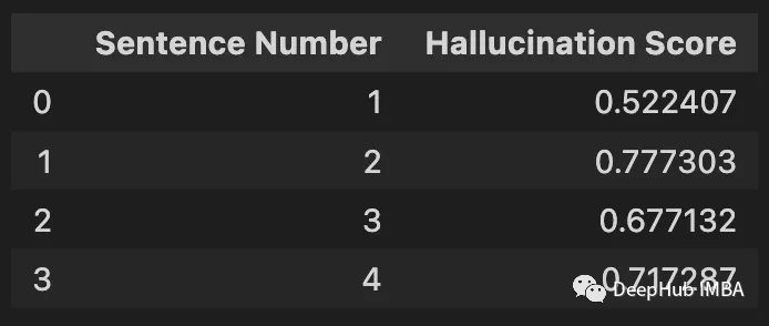
The illusion score for each sentence is obtained by subtracting 1 from each value above.
Compare the results with Nicolas Cage's answer.
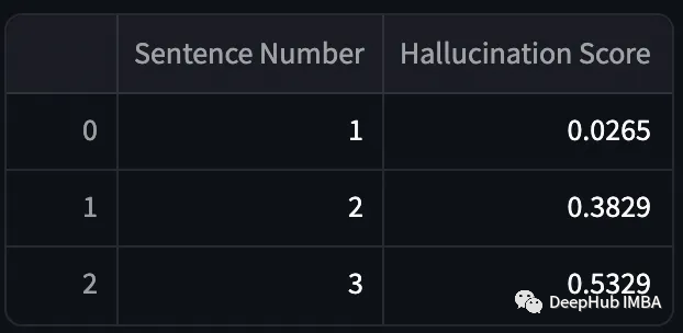
Valid outputs have lower hallucination scores, while fictional outputs have higher hallucination scores. But the process of calculating BERTScore is very time-consuming, which makes it unsuitable for real-time hallucination detection.
NLI
Natural Language Inference (NLI) involves determining whether a hypothesis logically follows or contradicts a given premise. This relationship can be classified as involved, ambivalent, or neutral. For NLI, we utilize the DeBERTa-v3-large model fine-tuned on the MNLI dataset to perform NLI.
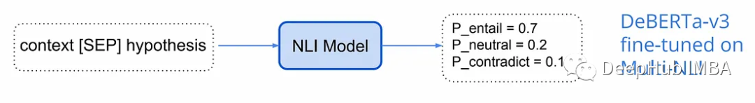
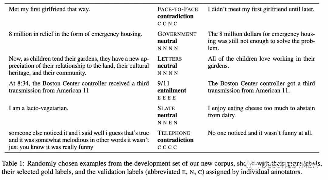
Below are some examples of premise-hypothesis pairs and their labels.
 def get_self_check_nli(output, sampled_passages):
     # spacy sentence tokenization
     sentences = [sent.text.strip() for sent in nlp(output).sents]
     selfcheck_nli = SelfCheckNLI(device=mps_device) # set device to 'cuda' if GPU is available
     sent_scores_nli = selfcheck_nli.predict(
         sentences = sentences, # list of sentences
         sampled_passages = sampled_passages, # list of sampled passages
     )
     df = pd.DataFrame({
     'Sentence Number': range(1, len(sent_scores_nli) + 1),
     'Probability of Contradiction': sent_scores_nli
     })
     return df
In the selfcheck_nli.predict function, each sentence in the original response is paired with each of the three samples.
 logits = model(**inputs).logits # neutral is already removed
 probs = torch.softmax(logits, dim=-1)
 prob_ = probs[0][1].item() # prob(contradiction)

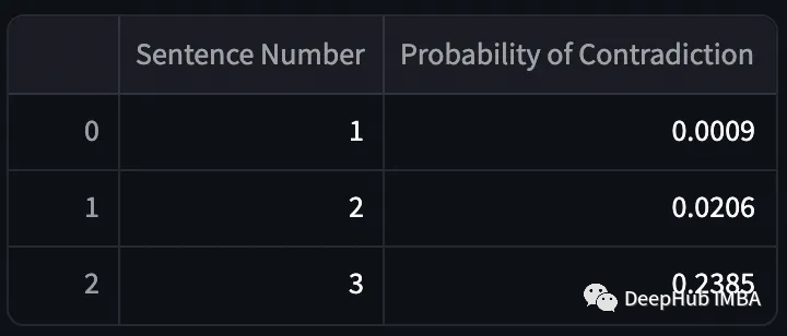
Now we repeat this process for each of the four sentences.

It can be seen that the probability of contradiction in the model output is very high. Now we compare it with the actual output.
The model did a great job! But the NLI check took a little too long.

Prompt
Newer approaches have begun to use llm itself to evaluate the generated text. Instead of using a formula to calculate the score, we send the output to gpt-3.5 turbo along with three samples. The model will determine how consistent the original output is relative to the other three samples generated.
 def llm_evaluate(sentences,sampled_passages):
     prompt = f"""You will be provided with a text passage \
                 and your task is to rate the consistency of that text to \
                 that of the provided context. Your answer must be only \
                 a number between 0.0 and 1.0 rounded to the nearest two \
                 decimal places where 0.0 represents no consistency and \
                 1.0 represents perfect consistency and similarity. \n\n \
                 Text passage: {sentences}. \n\n \
                 Context: {sampled_passages[0]} \n\n \
                 {sampled_passages[1]} \n\n \
                 {sampled_passages[2]}."""

     completion = client.chat.completions.create(
     model="gpt-3.5-turbo",
     messages=[
         {"role": "system", "content": ""},
         {"role": "user", "content": prompt}
     ]
     )

     return completion.choices[0].message.content
Evelyn Hartwell has a self-similarity score of 0. Nicolas Cage related output score is 0.95. The time required to earn a score is also low.

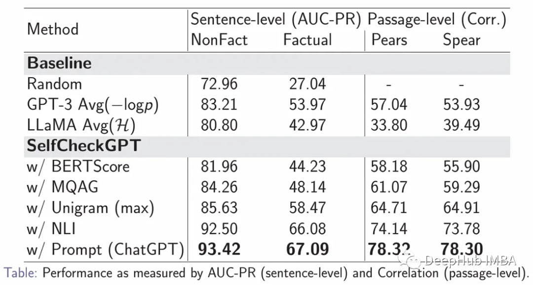
This seems to be the current best solution for the case, with Prompt significantly outperforming all other methods and NLI being the second best performing method.
The evaluation dataset was created by generating synthetic Wikipedia articles using the WikiBio dataset and GPT-3. To avoid vague concepts, the topics of the 238 articles were randomly selected from the top 20% of the longest articles. GPT-3 is prompted to generate the first paragraph for each concept in Wikipedia style.

, these generated paragraphs are manually annotated as facts at the sentence level. Each sentence is marked as majorly inaccurate, minorly inaccurate, or accurate. A total of 1908 sentences were annotated, approximately 40% of the sentences were majorly inaccurate, 33% of the sentences were minorly inaccurate, and 27% of the sentences were accurate.
To assess annotator consistency, 201 sentences were double annotated. If the annotators agree, that label is used; otherwise the worst-case label is chosen. Inter-annotator agreement measured by Cohen's kappa was 0.595 when choosing between accuracy, minor inaccuracy, and major inaccuracy, and 0.748 when minor/major inaccuracy was combined into one label.
The evaluation index AUC-PR refers to the area under the accuracy-recall curve and is an index used to evaluate the classification model.
Real-time hallucination detection
We can build a Streamlit application for real-time hallucination detection. As mentioned before, the best metric is the LLM self-similarity score. We will use a threshold of 0.5 to decide whether to display the generated output or the disclaimer.
 import streamlit as st
 import utils
 import pandas as pd

 # Streamlit app layout
 st.title('Anti-Hallucination Chatbot')

 # Text input
 user_input = st.text_input("Enter your text:")

 if user_input:

     prompt = user_input

     output, sampled_passages = utils.get_output_and_samples(prompt)

     # LLM score
     self_similarity_score = utils.llm_evaluate(output,sampled_passages)

     # Display the output
     st.write("**LLM output:**")
     if float(self_similarity_score) > 0.5:
         st.write(output)
     else:
         st.write("I'm sorry, but I don't have the specific information required to answer your question accurately. ")
Let's see the results.

Summarize
Hallucination detection in chatbots has been a long-discussed quality issue.
We only provide an overview of current research results: this is accomplished by generating multiple responses to the same prompt and comparing their consistency.
There is more work to be done, but rather than relying on human evaluation or hand-crafted rules, letting the model catch inconsistencies on its own seems to be a good direction.
Quote from this article:
https://avoid.overfit.cn/post/f32f440c1b99458e86d3e48c70ddcf94
Author: Iulia Brezeanu